Note
You can download this example as a Jupyter notebook or start it in interactive mode.
Meshed AC-DC example#
This example has a 3-node AC network coupled via AC-DC converters to a 3-node DC network. There is also a single point-to-point DC using the Link component.
The data files for this example are in the examples folder of the github repository: PyPSA/PyPSA.
[1]:
import pypsa
import numpy as np
import pandas as pd
import os
import matplotlib.pyplot as plt
import cartopy.crs as ccrs

%matplotlib inline
plt.rc("figure", figsize=(8, 8))
ERROR 1: PROJ: proj_create_from_database: Open of /home/docs/checkouts/readthedocs.org/user_builds/pypsa/conda/latest/share/proj failed
[2]:
network = pypsa.examples.ac_dc_meshed(from_master=True)
WARNING:pypsa.io:Importing network from PyPSA version v0.17.1 while current version is v0.27.1. Read the release notes at https://pypsa.readthedocs.io/en/latest/release_notes.html to prepare your network for import.
INFO:pypsa.io:Imported network ac-dc-meshed.nc has buses, carriers, generators, global_constraints, lines, links, loads
[3]:
# get current type (AC or DC) of the lines from the buses
lines_current_type = network.lines.bus0.map(network.buses.carrier)
lines_current_type
[3]:
Line
0    AC
1    AC
2    DC
3    DC
4    DC
5    AC
6    AC
Name: bus0, dtype: object
[4]:
network.plot(
    line_colors=lines_current_type.map(lambda ct: "r" if ct == "DC" else "b"),
    title="Mixed AC (blue) - DC (red) network - DC (cyan)",
    color_geomap=True,
    jitter=0.3,
)
plt.tight_layout()
/home/docs/checkouts/readthedocs.org/user_builds/pypsa/conda/latest/lib/python3.11/site-packages/cartopy/mpl/feature_artist.py:144: UserWarning: facecolor will have no effect as it has been defined as "never".
  warnings.warn('facecolor will have no effect as it has been '
/home/docs/checkouts/readthedocs.org/user_builds/pypsa/conda/latest/lib/python3.11/site-packages/cartopy/io/__init__.py:241: DownloadWarning: Downloading: https://naturalearth.s3.amazonaws.com/50m_physical/ne_50m_land.zip
  warnings.warn(f'Downloading: {url}', DownloadWarning)
/home/docs/checkouts/readthedocs.org/user_builds/pypsa/conda/latest/lib/python3.11/site-packages/cartopy/io/__init__.py:241: DownloadWarning: Downloading: https://naturalearth.s3.amazonaws.com/50m_physical/ne_50m_ocean.zip
  warnings.warn(f'Downloading: {url}', DownloadWarning)
/home/docs/checkouts/readthedocs.org/user_builds/pypsa/conda/latest/lib/python3.11/site-packages/cartopy/io/__init__.py:241: DownloadWarning: Downloading: https://naturalearth.s3.amazonaws.com/50m_cultural/ne_50m_admin_0_boundary_lines_land.zip
  warnings.warn(f'Downloading: {url}', DownloadWarning)
/home/docs/checkouts/readthedocs.org/user_builds/pypsa/conda/latest/lib/python3.11/site-packages/cartopy/io/__init__.py:241: DownloadWarning: Downloading: https://naturalearth.s3.amazonaws.com/50m_physical/ne_50m_coastline.zip
  warnings.warn(f'Downloading: {url}', DownloadWarning)

[5]:
network.links.loc["Norwich Converter", "p_nom_extendable"] = False
We inspect the topology of the network. Therefore use the function determine_network_topology and inspect the subnetworks in network.sub_networks.
[6]:
network.determine_network_topology()
network.sub_networks["n_branches"] = [
    len(sn.branches()) for sn in network.sub_networks.obj
]
network.sub_networks["n_buses"] = [len(sn.buses()) for sn in network.sub_networks.obj]

network.sub_networks
[6]:
| attribute | carrier | slack_bus | obj | n_branches | n_buses |
|---|---|---|---|---|---|
| SubNetwork | |||||
| 0 | AC | Manchester | SubNetwork 0 | 3 | 3 |
| 1 | DC | Norwich DC | SubNetwork 1 | 3 | 3 |
| 2 | AC | Frankfurt | SubNetwork 2 | 1 | 2 |
| 3 | AC | Norway | SubNetwork 3 | 0 | 1 |
The network covers 10 time steps. These are given by the snapshots attribute.
[7]:
network.snapshots
[7]:
DatetimeIndex(['2015-01-01 00:00:00', '2015-01-01 01:00:00',
               '2015-01-01 02:00:00', '2015-01-01 03:00:00',
               '2015-01-01 04:00:00', '2015-01-01 05:00:00',
               '2015-01-01 06:00:00', '2015-01-01 07:00:00',
               '2015-01-01 08:00:00', '2015-01-01 09:00:00'],
              dtype='datetime64[ns]', name='snapshot', freq=None)
There are 6 generators in the network, 3 wind and 3 gas. All are attached to buses:
[8]:
network.generators
[8]:
| bus | capital_cost | efficiency | marginal_cost | p_nom | p_nom_extendable | p_nom_min | carrier | control | type | ... | min_up_time | min_down_time | up_time_before | down_time_before | ramp_limit_up | ramp_limit_down | ramp_limit_start_up | ramp_limit_shut_down | weight | p_nom_opt | |
|---|---|---|---|---|---|---|---|---|---|---|---|---|---|---|---|---|---|---|---|---|---|
| Generator | |||||||||||||||||||||
| Manchester Wind | Manchester | 2793.651603 | 1.000000 | 0.110000 | 80.0 | True | 100.0 | wind | Slack | ... | 0 | 0 | 1 | 0 | NaN | NaN | 1.0 | 1.0 | 1.0 | 0.0 | |
| Manchester Gas | Manchester | 196.615168 | 0.350026 | 4.532368 | 50000.0 | True | 0.0 | gas | PQ | ... | 0 | 0 | 1 | 0 | NaN | NaN | 1.0 | 1.0 | 1.0 | 0.0 | |
| Norway Wind | Norway | 2184.374796 | 1.000000 | 0.090000 | 100.0 | True | 100.0 | wind | Slack | ... | 0 | 0 | 1 | 0 | NaN | NaN | 1.0 | 1.0 | 1.0 | 0.0 | |
| Norway Gas | Norway | 158.251250 | 0.356836 | 5.892845 | 20000.0 | True | 0.0 | gas | PQ | ... | 0 | 0 | 1 | 0 | NaN | NaN | 1.0 | 1.0 | 1.0 | 0.0 | |
| Frankfurt Wind | Frankfurt | 2129.456122 | 1.000000 | 0.100000 | 110.0 | True | 100.0 | wind | Slack | ... | 0 | 0 | 1 | 0 | NaN | NaN | 1.0 | 1.0 | 1.0 | 0.0 | |
| Frankfurt Gas | Frankfurt | 102.676953 | 0.351666 | 4.086322 | 80000.0 | True | 0.0 | gas | PQ | ... | 0 | 0 | 1 | 0 | NaN | NaN | 1.0 | 1.0 | 1.0 | 0.0 |
6 rows × 34 columns
We see that the generators have different capital and marginal costs. All of them have a p_nom_extendable set to True, meaning that capacities can be extended in the optimization.
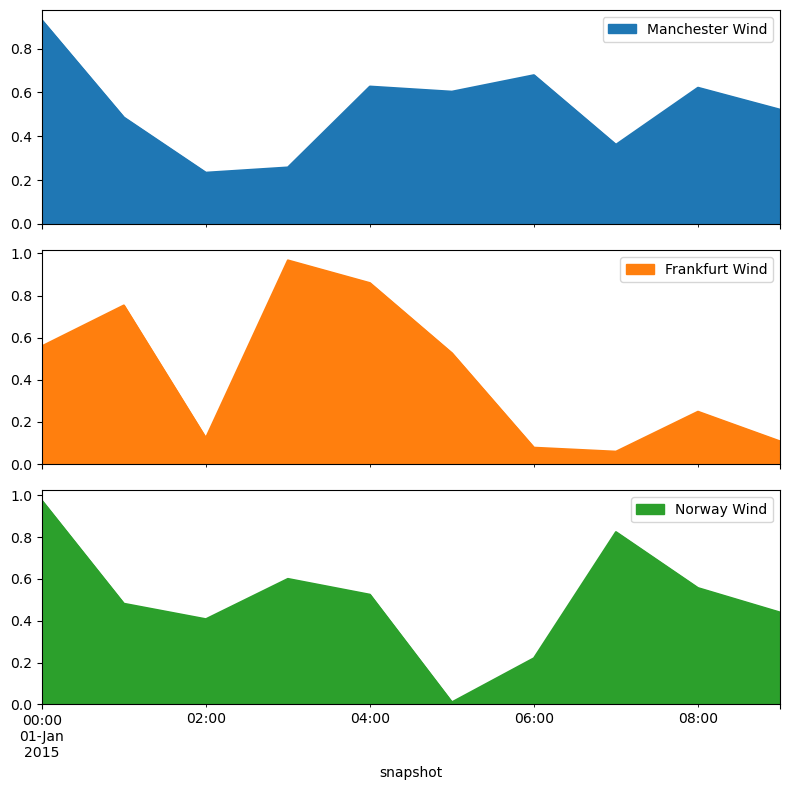
The wind generators have a per unit limit for each time step, given by the weather potentials at the site.
[9]:
network.generators_t.p_max_pu.plot.area(subplots=True)
plt.tight_layout()
Alright now we know how the network looks like, where the generators and lines are. Now, let’s perform a optimization of the operation and capacities.
[10]:
network.optimize();
WARNING:pypsa.components:The following lines have zero x, which could break the linear load flow:
Index(['2', '3', '4'], dtype='object', name='Line')
WARNING:pypsa.components:The following lines have zero r, which could break the linear load flow:
Index(['0', '1', '5', '6'], dtype='object', name='Line')
INFO:linopy.model: Solve problem using Glpk solver
INFO:linopy.io: Writing time: 0.08s
INFO:linopy.solvers:GLPSOL--GLPK LP/MIP Solver 5.0
Parameter(s) specified in the command line:
 --lp /tmp/linopy-problem-nh_sm23_.lp --output /tmp/linopy-solve-0ckd8ujw.sol
Reading problem data from '/tmp/linopy-problem-nh_sm23_.lp'...
467 rows, 187 columns, 986 non-zeros
2650 lines were read
GLPK Simplex Optimizer 5.0
467 rows, 187 columns, 986 non-zeros
Preprocessing...
371 rows, 186 columns, 890 non-zeros
Scaling...
 A: min|aij| =  9.693e-03  max|aij| =  1.215e+00  ratio =  1.254e+02
GM: min|aij| =  5.786e-01  max|aij| =  1.728e+00  ratio =  2.987e+00
EQ: min|aij| =  3.378e-01  max|aij| =  1.000e+00  ratio =  2.961e+00
Constructing initial basis...
Size of triangular part is 371
      0: obj =  -2.104300118e+07 inf =   9.187e+04 (92)
    165: obj =   8.711702088e+06 inf =   1.017e-11 (0) 1
*   245: obj =  -3.474094131e+06 inf =   0.000e+00 (0) 1
OPTIMAL LP SOLUTION FOUND
Time used:   0.0 secs
Memory used: 0.6 Mb (632037 bytes)
Writing basic solution to '/tmp/linopy-solve-0ckd8ujw.sol'...
INFO:linopy.constants: Optimization successful:
Status: ok
Termination condition: optimal
Solution: 187 primals, 467 duals
Objective: -3.47e+06
Solver model: not available
Solver message: optimal
/home/docs/checkouts/readthedocs.org/user_builds/pypsa/conda/latest/lib/python3.11/site-packages/pypsa/optimization/optimize.py:357: FutureWarning: A value is trying to be set on a copy of a DataFrame or Series through chained assignment using an inplace method.
The behavior will change in pandas 3.0. This inplace method will never work because the intermediate object on which we are setting values always behaves as a copy.

For example, when doing 'df[col].method(value, inplace=True)', try using 'df.method({col: value}, inplace=True)' or df[col] = df[col].method(value) instead, to perform the operation inplace on the original object.


  n.df(c)[attr + "_opt"].update(df)
INFO:pypsa.optimization.optimize:The shadow-prices of the constraints Generator-ext-p-lower, Generator-ext-p-upper, Line-ext-s-lower, Line-ext-s-upper, Link-fix-p-lower, Link-fix-p-upper, Link-ext-p-lower, Link-ext-p-upper, Kirchhoff-Voltage-Law were not assigned to the network.
The objective is given by:
[11]:
network.objective
[11]:
-3474094.131
Why is this number negative? It considers the starting point of the optimization, thus the existent capacities given by network.generators.p_nom are taken into account.
The real system cost are given by
[12]:
network.objective + network.objective_constant
[12]:
18440973.38727914
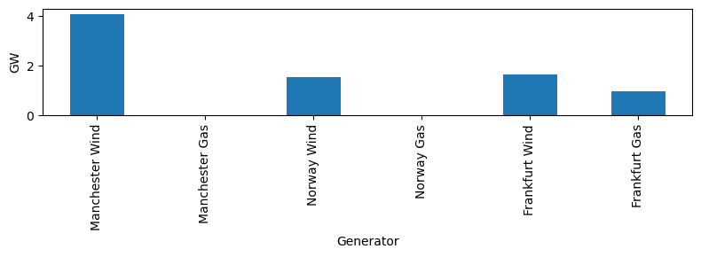
The optimal capacities are given by p_nom_opt for generators, links and storages and s_nom_opt for lines.
Let’s look how the optimal capacities for the generators look like.
[13]:
network.generators.p_nom_opt.div(1e3).plot.bar(ylabel="GW", figsize=(8, 3))
plt.tight_layout()
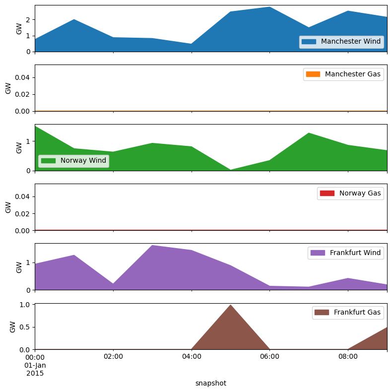
Their production is again given as a time-series in network.generators_t.
[14]:
network.generators_t.p.div(1e3).plot.area(subplots=True, ylabel="GW")
plt.tight_layout()
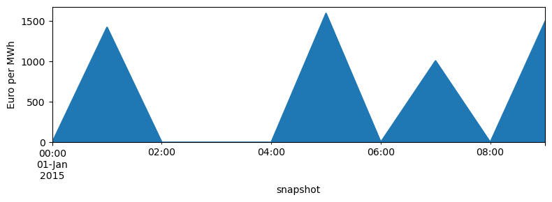
What are the Locational Marginal Prices in the network. From the optimization these are given for each bus and snapshot.
[15]:
network.buses_t.marginal_price.mean(1).plot.area(figsize=(8, 3), ylabel="Euro per MWh")
plt.tight_layout()
We can inspect further quantities as the active power of AC-DC converters and HVDC link.
[16]:
network.links_t.p0
[16]:
| Link | Norwich Converter | Norway Converter | Bremen Converter | DC link |
|---|---|---|---|---|
| snapshot | ||||
| 2015-01-01 00:00:00 | -250.8410 | 674.5850 | -423.7440 | -317.9980 |
| 2015-01-01 01:00:00 | 93.6719 | -116.7270 | 23.0553 | -96.6013 |
| 2015-01-01 02:00:00 | -285.2340 | 581.9710 | -296.7360 | 317.9980 |
| 2015-01-01 03:00:00 | -85.7721 | 272.5580 | -186.7860 | -317.9980 |
| 2015-01-01 04:00:00 | 317.3670 | -79.7495 | -237.6170 | -317.9980 |
| 2015-01-01 05:00:00 | 386.7480 | -494.1980 | 107.4500 | -317.9980 |
| 2015-01-01 06:00:00 | 900.0000 | -257.5210 | -642.4790 | 317.9980 |
| 2015-01-01 07:00:00 | 123.6770 | 971.9190 | -1095.6000 | -86.8587 |
| 2015-01-01 08:00:00 | 244.7160 | 850.8800 | -1095.6000 | 317.9980 |
| 2015-01-01 09:00:00 | 441.6100 | -86.8518 | -354.7580 | 294.7280 |
[17]:
network.lines_t.p0
[17]:
| Line | 0 | 1 | 2 | 3 | 4 | 5 | 6 |
|---|---|---|---|---|---|---|---|
| snapshot | |||||||
| 2015-01-01 00:00:00 | 79.4749 | -38.1056 | -52.9672 | -303.8080 | 370.7760 | -202.7270 | -534.341 |
| 2015-01-01 01:00:00 | -486.5070 | 749.9940 | -31.6237 | 62.0483 | -54.6789 | 393.7160 | -823.211 |
| 2015-01-01 02:00:00 | -287.6780 | 414.1490 | 10.1569 | -275.0770 | 306.8930 | 280.9070 | 173.898 |
| 2015-01-01 03:00:00 | -45.4725 | 234.4700 | -34.0407 | -119.8130 | 152.7450 | -232.7170 | -743.788 |
| 2015-01-01 04:00:00 | -73.2078 | 295.4210 | -227.1980 | 90.1683 | 10.4188 | -240.1060 | -883.818 |
| 2015-01-01 05:00:00 | -594.5000 | 1198.0800 | -125.9040 | 260.8440 | -233.3540 | 19.3590 | -1030.850 |
| 2015-01-01 06:00:00 | -661.2950 | 1378.4200 | -632.3710 | 267.6290 | 10.1079 | -53.4484 | 319.387 |
| 2015-01-01 07:00:00 | -383.7690 | 540.9070 | -469.9260 | -346.2480 | 625.6700 | 393.7160 | 600.729 |
| 2015-01-01 08:00:00 | -778.2810 | 1444.0700 | -522.1160 | -277.4000 | 573.4800 | 229.2940 | 501.346 |
| 2015-01-01 09:00:00 | -528.8910 | 836.2510 | -325.3130 | 116.2970 | 29.4448 | 393.7160 | -248.567 |
…or the active power injection per bus.
[18]:
network.buses_t.p
[18]:
| Bus | London | Norwich | Norwich DC | Manchester | Bremen | Bremen DC | Frankfurt | Norway | Norway DC |
|---|---|---|---|---|---|---|---|---|---|
| snapshot | |||||||||
| 2015-01-01 00:00:00 | 282.201756 | -164.621564 | -250.8410 | -117.580440 | -534.340378 | -423.7440 | 534.341153 | -0.000836 | 674.5850 |
| 2015-01-01 01:00:00 | -880.223261 | -356.278046 | 93.6719 | 1236.500376 | -823.210934 | 23.0553 | 823.213894 | -0.000047 | -116.7270 |
| 2015-01-01 02:00:00 | -568.585312 | -133.242353 | -285.2340 | 701.827124 | 173.897870 | -296.7360 | -173.897928 | -0.000744 | 581.9710 |
| 2015-01-01 03:00:00 | 187.244855 | -467.187439 | -85.7721 | 279.942178 | -743.788306 | -186.7860 | 743.788236 | -0.000233 | 272.5580 |
| 2015-01-01 04:00:00 | 166.897831 | -535.526858 | 317.3670 | 368.629241 | -883.817781 | -237.6170 | 883.819245 | -0.000373 | -79.7495 |
| 2015-01-01 05:00:00 | -613.859052 | -1178.724266 | 386.7480 | 1792.586681 | -1030.848687 | 107.4500 | 1030.848757 | 0.000251 | -494.1980 |
| 2015-01-01 06:00:00 | -607.846287 | -1431.870681 | 900.0000 | 2039.712900 | 319.386410 | -642.4790 | -319.386752 | 0.000035 | -257.5210 |
| 2015-01-01 07:00:00 | -777.484622 | -147.190467 | 123.6770 | 924.675111 | 600.732759 | -1095.6000 | -600.728866 | -0.001450 | 971.9190 |
| 2015-01-01 08:00:00 | -1007.575264 | -1214.775068 | 244.7160 | 2222.351918 | 501.350224 | -1095.6000 | -501.346780 | 0.000507 | 850.8800 |
| 2015-01-01 09:00:00 | -922.606986 | -442.534834 | 441.6100 | 1365.139414 | -248.567092 | -354.7580 | 248.567354 | -0.000377 | -86.8518 |