Note
You can download this example as a Jupyter notebook or start it in interactive mode.
Battery Electric Vehicle Charging#
In this example a battery electric vehicle (BEV) is driven 100 km in the morning and 100 km in the evening, to simulate commuting, and charged during the day by a solar panel at the driver’s place of work. The size of the panel is computed by the optimisation.
The BEV has a battery of size 100 kWh and an electricity consumption of 0.18 kWh/km.
NB: this example will use units of kW and kWh, unlike the PyPSA defaults
[1]:
import pypsa
import pandas as pd
import matplotlib.pyplot as plt

%matplotlib inline
ERROR 1: PROJ: proj_create_from_database: Open of /home/docs/checkouts/readthedocs.org/user_builds/pypsa/conda/latest/share/proj failed
[2]:
# use 24 hour period for consideration
index = pd.date_range("2016-01-01 00:00", "2016-01-01 23:00", freq="H")

# consumption pattern of BEV
bev_usage = pd.Series([0.0] * 7 + [9.0] * 2 + [0.0] * 8 + [9.0] * 2 + [0.0] * 5, index)

# solar PV panel generation per unit of capacity
pv_pu = pd.Series(
    [0.0] * 7
    + [0.2, 0.4, 0.6, 0.75, 0.85, 0.9, 0.85, 0.75, 0.6, 0.4, 0.2, 0.1]
    + [0.0] * 5,
    index,
)

# availability of charging - i.e. only when parked at office
charger_p_max_pu = pd.Series(0, index=index)
charger_p_max_pu["2016-01-01 09:00":"2016-01-01 16:00"] = 1.0
/tmp/ipykernel_3179/2212892536.py:2: FutureWarning: 'H' is deprecated and will be removed in a future version, please use 'h' instead.
  index = pd.date_range("2016-01-01 00:00", "2016-01-01 23:00", freq="H")
[3]:
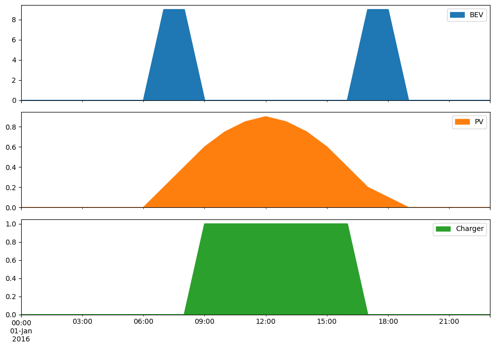
df = pd.concat({"BEV": bev_usage, "PV": pv_pu, "Charger": charger_p_max_pu}, axis=1)
df.plot.area(subplots=True, figsize=(10, 7))
plt.tight_layout()
Initialize the network
[4]:
network = pypsa.Network()
network.set_snapshots(index)

network.add("Bus", "place of work", carrier="AC")

network.add("Bus", "battery", carrier="Li-ion")

network.add(
    "Generator",
    "PV panel",
    bus="place of work",
    p_nom_extendable=True,
    p_max_pu=pv_pu,
    capital_cost=1000.0,
)

network.add("Load", "driving", bus="battery", p_set=bev_usage)

network.add(
    "Link",
    "charger",
    bus0="place of work",
    bus1="battery",
    p_nom=120,  # super-charger with 120 kW
    p_max_pu=charger_p_max_pu,
    efficiency=0.9,
)


network.add("Store", "battery storage", bus="battery", e_cyclic=True, e_nom=100.0)
[5]:
network.optimize()
print("Objective:", network.objective)
INFO:linopy.model: Solve problem using Glpk solver
INFO:linopy.io: Writing time: 0.04s
INFO:linopy.solvers:GLPSOL--GLPK LP/MIP Solver 5.0
Parameter(s) specified in the command line:
 --lp /tmp/linopy-problem-qrx2zyuc.lp --output /tmp/linopy-solve-euz2wp4i.sol
Reading problem data from '/tmp/linopy-problem-qrx2zyuc.lp'...
217 rows, 97 columns, 325 non-zeros
1078 lines were read
GLPK Simplex Optimizer 5.0
217 rows, 97 columns, 325 non-zeros
Preprocessing...
48 rows, 49 columns, 104 non-zeros
Scaling...
 A: min|aij| =  4.000e-01  max|aij| =  1.000e+00  ratio =  2.500e+00
Problem data seem to be well scaled
Constructing initial basis...
Size of triangular part is 47
      0: obj =   0.000000000e+00 inf =   4.140e+02 (17)
      8: obj =   1.818181818e+04 inf =   0.000e+00 (0)
*    13: obj =   7.017543860e+03 inf =   0.000e+00 (0)
OPTIMAL LP SOLUTION FOUND
Time used:   0.0 secs
Memory used: 0.2 Mb (173076 bytes)
Writing basic solution to '/tmp/linopy-solve-euz2wp4i.sol'...
INFO:linopy.constants: Optimization successful:
Status: ok
Termination condition: optimal
Solution: 97 primals, 217 duals
Objective: 7.02e+03
Solver model: not available
Solver message: optimal
/home/docs/checkouts/readthedocs.org/user_builds/pypsa/conda/latest/lib/python3.11/site-packages/pypsa/optimization/optimize.py:357: FutureWarning: A value is trying to be set on a copy of a DataFrame or Series through chained assignment using an inplace method.
The behavior will change in pandas 3.0. This inplace method will never work because the intermediate object on which we are setting values always behaves as a copy.

For example, when doing 'df[col].method(value, inplace=True)', try using 'df.method({col: value}, inplace=True)' or df[col] = df[col].method(value) instead, to perform the operation inplace on the original object.


  n.df(c)[attr + "_opt"].update(df)
INFO:pypsa.optimization.optimize:The shadow-prices of the constraints Generator-ext-p-lower, Generator-ext-p-upper, Link-fix-p-lower, Link-fix-p-upper, Store-fix-e-lower, Store-fix-e-upper, Store-energy_balance were not assigned to the network.
Objective: 7017.54386
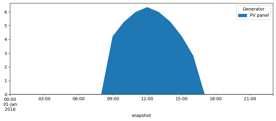
The optimal panel size in kW is
[6]:
network.generators.p_nom_opt["PV panel"]
[6]:
7.01754
[7]:
network.generators_t.p.plot.area(figsize=(9, 4))
plt.tight_layout()
[8]:
df = pd.DataFrame(
    {attr: network.stores_t[attr]["battery storage"] for attr in ["p", "e"]}
)
df.plot(grid=True, figsize=(10, 5))
plt.legend(labels=["Energy output", "State of charge"])
plt.tight_layout()
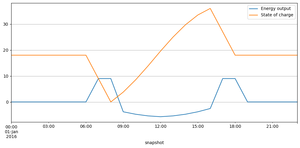
The losses in kWh per pay are:
[9]:
(
    network.generators_t.p.loc[:, "PV panel"].sum()
    - network.loads_t.p.loc[:, "driving"].sum()
)
[9]:
4.000010000000003
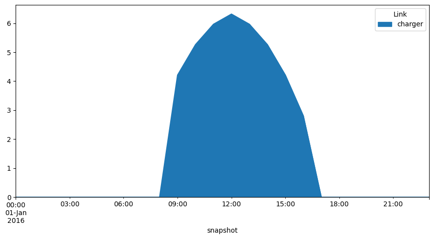
[10]:
network.links_t.p0.plot.area(figsize=(9, 5))
plt.tight_layout()