Note

You can download this example as a Jupyter notebook or start it in interactive mode.

Two chained reservoirs

Two disconnected electrical loads are fed from two reservoirs linked by a river; the first reservoir has inflow from rain onto a water basin.

Note that the two reservoirs are tightly coupled, meaning there is no time delay between the first one emptying and the second one filling, as there would be if there were a long stretch of river between the reservoirs. The reservoirs are essentially assumed to be close to each other. A time delay would require a “Link” element between different snapshots, which is not yet supported by PyPSA (but could be enabled by passing network.optimize() an extra_functionality function).

import pypsa
import pandas as pd
import numpy as np
import matplotlib.pyplot as plt

ERROR 1: PROJ: proj_create_from_database: Open of /home/docs/checkouts/readthedocs.org/user_builds/pypsa/conda/latest/share/proj failed

network = pypsa.Network()
network.set_snapshots(pd.date_range("2016-01-01 00:00", "2016-01-01 03:00", freq="H"))

/tmp/ipykernel_3466/447536113.py:2: FutureWarning: 'H' is deprecated and will be removed in a future version, please use 'h' instead.
  network.set_snapshots(pd.date_range("2016-01-01 00:00", "2016-01-01 03:00", freq="H"))

Add assets to the network.

network.add("Carrier", "reservoir")
network.add("Carrier", "rain")

network.add("Bus", "0", carrier="AC")
network.add("Bus", "1", carrier="AC")

network.add("Bus", "0 reservoir", carrier="reservoir")
network.add("Bus", "1 reservoir", carrier="reservoir")


network.add(
    "Generator",
    "rain",
    bus="0 reservoir",
    carrier="rain",
    p_nom=1000,
    p_max_pu=[0.0, 0.2, 0.7, 0.4],
)


network.add("Load", "0 load", bus="0", p_set=20.0)

network.add("Load", "1 load", bus="1", p_set=30.0)

The efficiency of a river is the relation between the gravitational potential energy of 1 m^3 of water in reservoir 0 relative to its turbine versus the potential energy of 1 m^3 of water in reservoir 1 relative to its turbine

network.add(
    "Link",
    "spillage",
    bus0="0 reservoir",
    bus1="1 reservoir",
    efficiency=0.5,
    p_nom_extendable=True,
)


# water from turbine also goes into next reservoir
network.add(
    "Link",
    "0 turbine",
    bus0="0 reservoir",
    bus1="0",
    bus2="1 reservoir",
    efficiency=0.9,
    efficiency2=0.5,
    capital_cost=1000,
    p_nom_extendable=True,
)

network.add(
    "Link",
    "1 turbine",
    bus0="1 reservoir",
    bus1="1",
    efficiency=0.9,
    capital_cost=1000,
    p_nom_extendable=True,
)


network.add(
    "Store", "0 reservoir", bus="0 reservoir", e_cyclic=True, e_nom_extendable=True
)

network.add(
    "Store", "1 reservoir", bus="1 reservoir", e_cyclic=True, e_nom_extendable=True
)

network.optimize(network.snapshots)
print("Objective:", network.objective)

WARNING:pypsa.components:The following links have bus2 which are not defined:
Index(['spillage'], dtype='object', name='Link')

WARNING:pypsa.components:The following links have bus2 which are not defined:
Index(['spillage'], dtype='object', name='Link')

INFO:linopy.model: Solve problem using Glpk solver

INFO:linopy.io: Writing time: 0.05s

INFO:linopy.solvers:GLPSOL--GLPK LP/MIP Solver 5.0
Parameter(s) specified in the command line:
 --lp /tmp/linopy-problem-jfnwk787.lp --output /tmp/linopy-solve-7u3fgme_.sol
Reading problem data from '/tmp/linopy-problem-jfnwk787.lp'...
77 rows, 37 columns, 137 non-zeros
410 lines were read
GLPK Simplex Optimizer 5.0
77 rows, 37 columns, 137 non-zeros
Preprocessing...
28 rows, 23 columns, 64 non-zeros
Scaling...
 A: min|aij| =  5.000e-01  max|aij| =  1.000e+00  ratio =  2.000e+00
Problem data seem to be well scaled
Constructing initial basis...
Size of triangular part is 28
      0: obj =   5.555555556e+04 inf =   2.222e+02 (5)
      6: obj =   5.555555556e+04 inf =   0.000e+00 (0)
OPTIMAL LP SOLUTION FOUND
Time used:   0.0 secs
Memory used: 0.1 Mb (80884 bytes)
Writing basic solution to '/tmp/linopy-solve-7u3fgme_.sol'...

INFO:linopy.constants: Optimization successful:
Status: ok
Termination condition: optimal
Solution: 37 primals, 77 duals
Objective: 5.56e+04
Solver model: not available
Solver message: optimal

/home/docs/checkouts/readthedocs.org/user_builds/pypsa/conda/latest/lib/python3.11/site-packages/pypsa/optimization/optimize.py:357: FutureWarning: A value is trying to be set on a copy of a DataFrame or Series through chained assignment using an inplace method.
The behavior will change in pandas 3.0. This inplace method will never work because the intermediate object on which we are setting values always behaves as a copy.

For example, when doing 'df[col].method(value, inplace=True)', try using 'df.method({col: value}, inplace=True)' or df[col] = df[col].method(value) instead, to perform the operation inplace on the original object.


  n.df(c)[attr + "_opt"].update(df)
INFO:pypsa.optimization.optimize:The shadow-prices of the constraints Generator-fix-p-lower, Generator-fix-p-upper, Link-ext-p-lower, Link-ext-p-upper, Store-ext-e-lower, Store-ext-e-upper, Store-energy_balance were not assigned to the network.

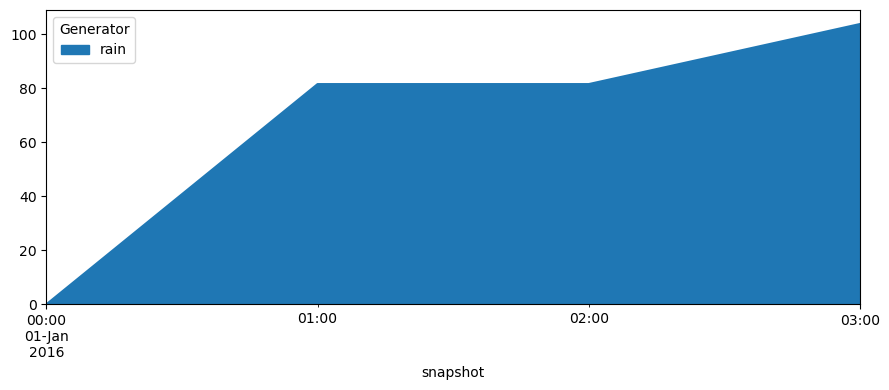
Objective: 55555.55556

network.generators_t.p.plot.area(figsize=(9, 4))
plt.tight_layout()

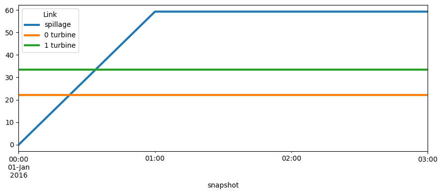
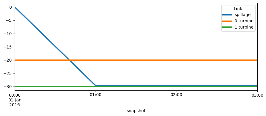
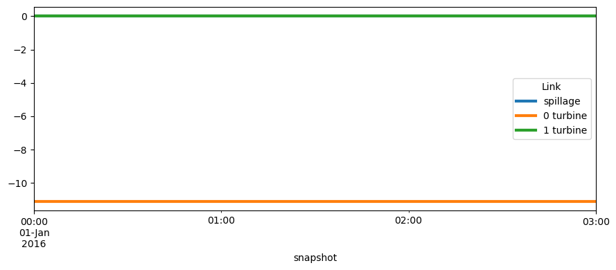
Now, let’s have look at the different outputs of the links.

network.links_t.p0.plot(figsize=(9, 4), lw=3)
plt.tight_layout()

network.links_t.p1.plot(figsize=(9, 4), lw=3)
plt.tight_layout()

network.links_t.p2.plot(figsize=(9, 4), lw=3)
plt.tight_layout()

What are the energy outputs and energy levels at the reservoirs?

pd.DataFrame({attr: network.stores_t[attr]["0 reservoir"] for attr in ["p", "e"]})

	p	e
snapshot
2016-01-01 00:00:00	22.2222	0.0000
2016-01-01 01:00:00	0.0000	0.0000
2016-01-01 02:00:00	0.0000	0.0000
2016-01-01 03:00:00	-22.2222	22.2222

pd.DataFrame({attr: network.stores_t[attr]["1 reservoir"] for attr in ["p", "e"]})

	p	e
snapshot
2016-01-01 00:00:00	22.22220	0.00000
2016-01-01 01:00:00	-7.40741	7.40741
2016-01-01 02:00:00	-7.40741	14.81480
2016-01-01 03:00:00	-7.40741	22.22220