Note
You can download this example as a Jupyter notebook or start it in interactive mode.
Flow Plot Example#
Here, we are going to import a network and plot the electricity flow
[1]:
import pypsa, os
import cartopy.crs as ccrs
import matplotlib.pyplot as plt
import pandas as pd

import warnings
from shapely.errors import ShapelyDeprecationWarning

warnings.filterwarnings("ignore", category=ShapelyDeprecationWarning)
plt.rc("figure", figsize=(10, 8))
ERROR 1: PROJ: proj_create_from_database: Open of /home/docs/checkouts/readthedocs.org/user_builds/pypsa/conda/latest/share/proj failed
Import and optimize a network#
[2]:
n = pypsa.examples.ac_dc_meshed(from_master=True)
n.optimize()
WARNING:pypsa.io:Importing network from PyPSA version v0.17.1 while current version is v0.27.1. Read the release notes at https://pypsa.readthedocs.io/en/latest/release_notes.html to prepare your network for import.
INFO:pypsa.io:Imported network ac-dc-meshed.nc has buses, carriers, generators, global_constraints, lines, links, loads
WARNING:pypsa.components:The following lines have zero x, which could break the linear load flow:
Index(['2', '3', '4'], dtype='object', name='Line')
WARNING:pypsa.components:The following lines have zero r, which could break the linear load flow:
Index(['0', '1', '5', '6'], dtype='object', name='Line')
INFO:linopy.model: Solve problem using Glpk solver
INFO:linopy.io: Writing time: 0.13s
INFO:linopy.solvers:GLPSOL--GLPK LP/MIP Solver 5.0
Parameter(s) specified in the command line:
 --lp /tmp/linopy-problem-4hte_0o4.lp --output /tmp/linopy-solve-wevjj_0n.sol
Reading problem data from '/tmp/linopy-problem-4hte_0o4.lp'...
468 rows, 188 columns, 1007 non-zeros
2678 lines were read
GLPK Simplex Optimizer 5.0
468 rows, 188 columns, 1007 non-zeros
Preprocessing...
391 rows, 187 columns, 930 non-zeros
Scaling...
 A: min|aij| =  9.693e-03  max|aij| =  1.215e+00  ratio =  1.254e+02
GM: min|aij| =  5.786e-01  max|aij| =  1.728e+00  ratio =  2.987e+00
EQ: min|aij| =  3.377e-01  max|aij| =  1.000e+00  ratio =  2.961e+00
Constructing initial basis...
Size of triangular part is 391
      0: obj =  -2.104321118e+07 inf =   9.486e+04 (101)
    162: obj =   1.210828068e+07 inf =   1.864e-11 (0) 1
*   239: obj =  -3.474256041e+06 inf =   1.755e-12 (0) 1
OPTIMAL LP SOLUTION FOUND
Time used:   0.0 secs
Memory used: 0.6 Mb (656771 bytes)
Writing basic solution to '/tmp/linopy-solve-wevjj_0n.sol'...
INFO:linopy.constants: Optimization successful:
Status: ok
Termination condition: optimal
Solution: 188 primals, 468 duals
Objective: -3.47e+06
Solver model: not available
Solver message: optimal
/home/docs/checkouts/readthedocs.org/user_builds/pypsa/conda/latest/lib/python3.11/site-packages/pypsa/optimization/optimize.py:357: FutureWarning: A value is trying to be set on a copy of a DataFrame or Series through chained assignment using an inplace method.
The behavior will change in pandas 3.0. This inplace method will never work because the intermediate object on which we are setting values always behaves as a copy.

For example, when doing 'df[col].method(value, inplace=True)', try using 'df.method({col: value}, inplace=True)' or df[col] = df[col].method(value) instead, to perform the operation inplace on the original object.


  n.df(c)[attr + "_opt"].update(df)
INFO:pypsa.optimization.optimize:The shadow-prices of the constraints Generator-ext-p-lower, Generator-ext-p-upper, Line-ext-s-lower, Line-ext-s-upper, Link-ext-p-lower, Link-ext-p-upper, Kirchhoff-Voltage-Law were not assigned to the network.
[2]:
('ok', 'optimal')
Get mean generator power by bus and carrier:
[3]:
gen = n.generators.assign(g=n.generators_t.p.mean()).groupby(["bus", "carrier"]).g.sum()
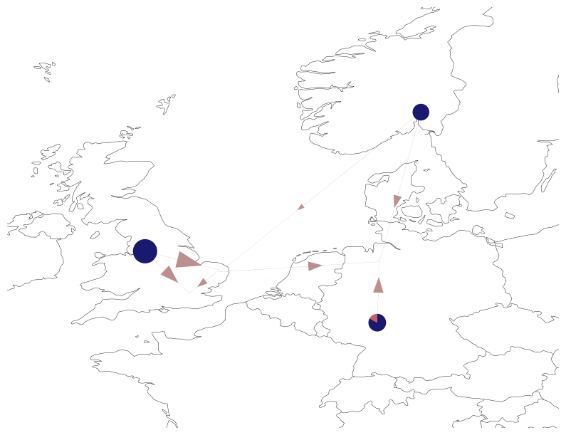
Plot the electricity flows:
[4]:
# links are not displayed for prettier output ('link_widths=0')
n.plot(
    bus_sizes=gen / 5e3,
    bus_colors={"gas": "indianred", "wind": "midnightblue"},
    margin=0.5,
    flow="mean",
    line_widths=0.1,
    link_widths=0,
)
plt.show()
/home/docs/checkouts/readthedocs.org/user_builds/pypsa/conda/latest/lib/python3.11/site-packages/cartopy/mpl/feature_artist.py:144: UserWarning: facecolor will have no effect as it has been defined as "never".
  warnings.warn('facecolor will have no effect as it has been '
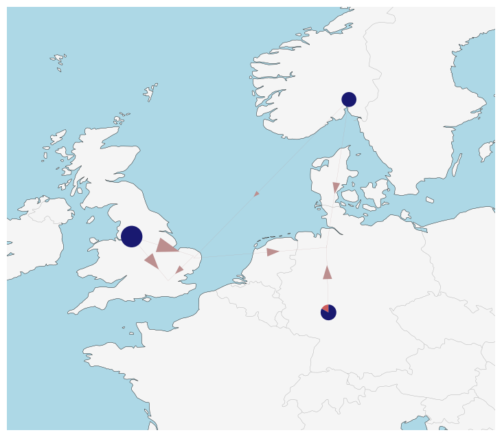
Plot the electricity flows with a different projection and a colored map:
[5]:
# links are not displayed for prettier output ('link_widths=0')
n.plot(
    bus_sizes=gen / 5e3,
    bus_colors={"gas": "indianred", "wind": "midnightblue"},
    margin=0.5,
    flow="mean",
    line_widths=0.1,
    link_widths=0,
    projection=ccrs.EqualEarth(),
    color_geomap=True,
)
plt.show()
/home/docs/checkouts/readthedocs.org/user_builds/pypsa/conda/latest/lib/python3.11/site-packages/cartopy/mpl/feature_artist.py:144: UserWarning: facecolor will have no effect as it has been defined as "never".
  warnings.warn('facecolor will have no effect as it has been '
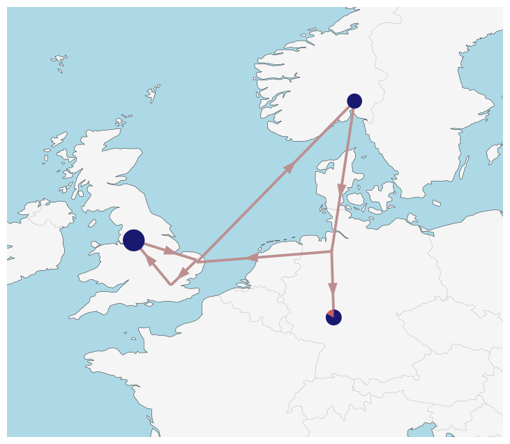
Set arbitrary values as flow argument using the MultiIndex of n.branches():
[6]:
flow = pd.Series(10, index=n.branches().index)
[7]:
flow
[7]:
component  name
Line       0                    10
           1                    10
           2                    10
           3                    10
           4                    10
           5                    10
           6                    10
Link       Norwich Converter    10
           Norway Converter     10
           Bremen Converter     10
           DC link              10
dtype: int64
[8]:
# links are not displayed for prettier output ('link_widths=0')
n.plot(
    bus_sizes=gen / 5e3,
    bus_colors={"gas": "indianred", "wind": "midnightblue"},
    margin=0.5,
    flow=flow,
    line_widths=2.7,
    link_widths=0,
    projection=ccrs.EqualEarth(),
    color_geomap=True,
)
plt.show()
/home/docs/checkouts/readthedocs.org/user_builds/pypsa/conda/latest/lib/python3.11/site-packages/cartopy/mpl/feature_artist.py:144: UserWarning: facecolor will have no effect as it has been defined as "never".
  warnings.warn('facecolor will have no effect as it has been '
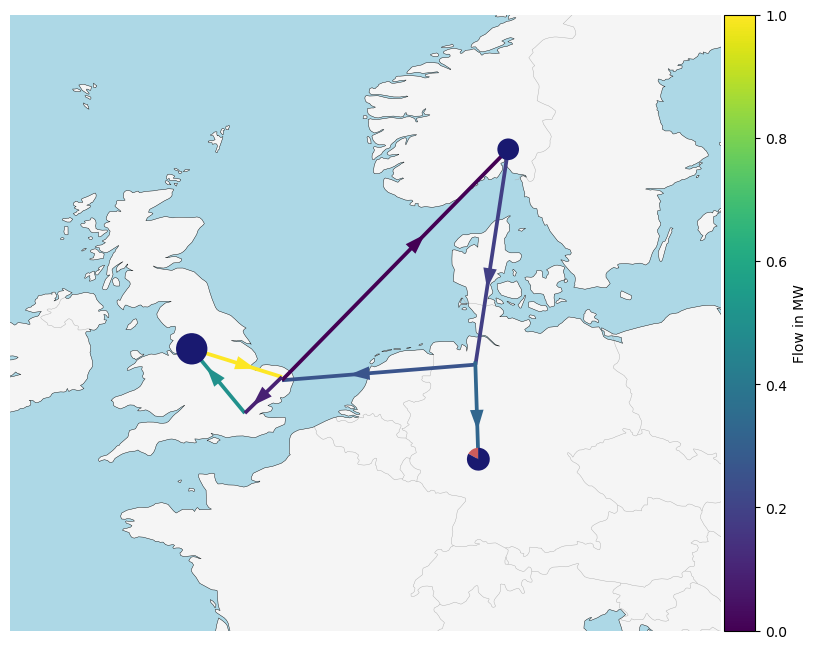
Adjust link colors according to their mean load:
[9]:
# Pandas series with MultiIndex
# links are not displayed for prettier output ('link_widths=0')
collection = n.plot(
    bus_sizes=gen / 5e3,
    bus_colors={"gas": "indianred", "wind": "midnightblue"},
    margin=0.5,
    flow=flow,
    line_widths=2.7,
    link_widths=0,
    projection=ccrs.EqualEarth(),
    color_geomap=True,
    line_colors=n.lines_t.p0.mean().abs(),
)

plt.colorbar(collection[2], fraction=0.04, pad=0.004, label="Flow in MW")
plt.show()
/home/docs/checkouts/readthedocs.org/user_builds/pypsa/conda/latest/lib/python3.11/site-packages/cartopy/mpl/feature_artist.py:144: UserWarning: facecolor will have no effect as it has been defined as "never".
  warnings.warn('facecolor will have no effect as it has been '