Note

You can download this example as a Jupyter notebook or start it in interactive mode.

Screening curve analysis#

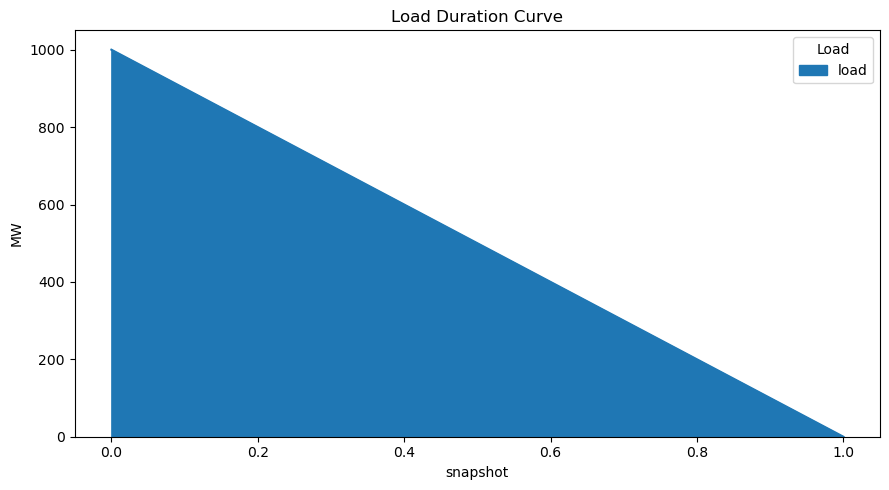
Compute the long-term equilibrium power plant investment for a given load duration curve (1000-1000z for z \(\in\) [0,1]) and a given set of generator investment options.

[1]:

import pypsa
import numpy as np
import pandas as pd
import matplotlib.pyplot as plt

ERROR 1: PROJ: proj_create_from_database: Open of /home/docs/checkouts/readthedocs.org/user_builds/pypsa/conda/latest/share/proj failed

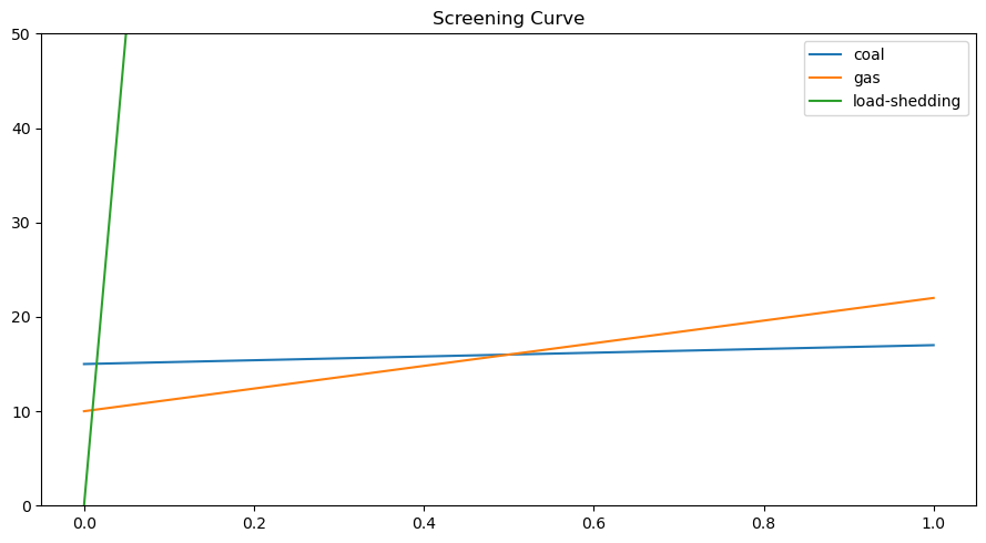
Generator marginal (m) and capital (c) costs in EUR/MWh - numbers chosen for simple answer.

[2]:

generators = {
    "coal": {"m": 2, "c": 15},
    "gas": {"m": 12, "c": 10},
    "load-shedding": {"m": 1012, "c": 0},
}

The screening curve intersections are at 0.01 and 0.5.

[3]:

x = np.linspace(0, 1, 101)
df = pd.DataFrame(
    {key: pd.Series(item["c"] + x * item["m"], x) for key, item in generators.items()}
)
df.plot(ylim=[0, 50], title="Screening Curve", figsize=(9, 5))
plt.tight_layout()

../_images/examples_generation-investment-screening-curve_5_0.png

[4]:

n = pypsa.Network()

num_snapshots = 1001
n.snapshots = np.linspace(0, 1, num_snapshots)
n.snapshot_weightings = n.snapshot_weightings / num_snapshots

n.add("Bus", name="bus")

n.add("Load", name="load", bus="bus", p_set=1000 - 1000 * n.snapshots.values)

for gen in generators:
    n.add(
        "Generator",
        name=gen,
        bus="bus",
        p_nom_extendable=True,
        marginal_cost=float(generators[gen]["m"]),
        capital_cost=float(generators[gen]["c"]),
    )

[5]:

n.loads_t.p_set.plot.area(title="Load Duration Curve", figsize=(9, 5), ylabel="MW")
plt.tight_layout()

../_images/examples_generation-investment-screening-curve_7_0.png

[6]:

n.optimize(solver_name="cbc")
n.objective

INFO:linopy.model: Solve problem using Cbc solver

INFO:linopy.io: Writing time: 0.06s

INFO:linopy.solvers:Welcome to the CBC MILP Solver
Version: 2.10.10
Build Date: Apr 19 2023

command line - cbc -printingOptions all -import /tmp/linopy-problem-vr3oco_6.lp -solve -solu /tmp/linopy-solve-f1ls0wyv.sol (default strategy 1)
Option for printingOptions changed from normal to all
Presolve 3000 (-4010) rows, 3002 (-4) columns and 7000 (-5015) elements
Perturbing problem by 0.001% of 15 - largest nonzero change 0.00017295671 ( 2.8764424%) - largest zero change 0
0  Obj 0 Primal inf 500500 (1000)
135  Obj 257.11517 Primal inf 500500 (1000)
270  Obj 476.8907 Primal inf 500500 (1000)
405  Obj 1212.8467 Primal inf 500500 (1000)
540  Obj 1991.8018 Primal inf 500500 (1000)
675  Obj 12597.874 Primal inf 306936 (783)
810  Obj 13245.075 Primal inf 248160 (704)
945  Obj 13823.496 Primal inf 195625 (625)
1080  Obj 14337.966 Primal inf 148785 (545)
1215  Obj 14637.617 Primal inf 44253 (297)
1350  Obj 14700.997 Primal inf 13203 (162)
1485  Obj 14727.167 Primal inf 377.99997 (27)
1512  Obj 14727.938
Optimal - objective value 14706.194
After Postsolve, objective 14706.194, infeasibilities - dual 0 (0), primal 0 (0)
Optimal objective 14706.19381 - 1512 iterations time 0.052, Presolve 0.02
Total time (CPU seconds):       0.14   (Wallclock seconds):       0.07

INFO:linopy.constants: Optimization successful:
Status: ok
Termination condition: optimal
Solution: 3006 primals, 7010 duals
Objective: 1.47e+04
Solver model: not available
Solver message: Optimal - objective value 14706.19380619

/home/docs/checkouts/readthedocs.org/user_builds/pypsa/conda/latest/lib/python3.11/site-packages/pypsa/optimization/optimize.py:357: FutureWarning: A value is trying to be set on a copy of a DataFrame or Series through chained assignment using an inplace method.
The behavior will change in pandas 3.0. This inplace method will never work because the intermediate object on which we are setting values always behaves as a copy.

For example, when doing 'df[col].method(value, inplace=True)', try using 'df.method({col: value}, inplace=True)' or df[col] = df[col].method(value) instead, to perform the operation inplace on the original object.


  n.df(c)[attr + "_opt"].update(df)
INFO:pypsa.optimization.optimize:The shadow-prices of the constraints Generator-ext-p-lower, Generator-ext-p-upper were not assigned to the network.

[6]:

14706.19380619

The capacity is set by total electricity required.

NB: No load shedding since all prices are below 10 000.

[7]:

n.generators.p_nom_opt.round(2)

[7]:

Generator
coal             500.0
gas              490.0
load-shedding     10.0
Name: p_nom_opt, dtype: float64

[8]:

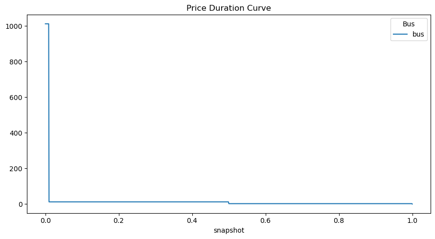
n.buses_t.marginal_price.plot(title="Price Duration Curve", figsize=(9, 4))
plt.tight_layout()

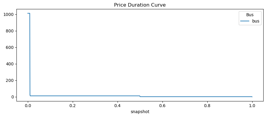
../_images/examples_generation-investment-screening-curve_11_0.png

The prices correspond either to VOLL (1012) for first 0.01 or the marginal costs (12 for 0.49 and 2 for 0.5)

Except for (infinitesimally small) points at the screening curve intersections, which correspond to changing the load duration near the intersection, so that capacity changes. This explains 7 = (12+10 - 15) (replacing coal with gas) and 22 = (12+10) (replacing load-shedding with gas).

Note: What remains unclear is what is causing :nbsphinx-math:`l `= 0… it should be 2.

[9]:

n.buses_t.marginal_price.round(2).sum(axis=1).value_counts()

[9]:

2.0       499
12.0      489
1012.0     10
22.0        1
7.0         1
0.0         1
Name: count, dtype: int64

[10]:

n.generators_t.p.plot(ylim=[0, 600], title="Generation Dispatch", figsize=(9, 5))
plt.tight_layout()

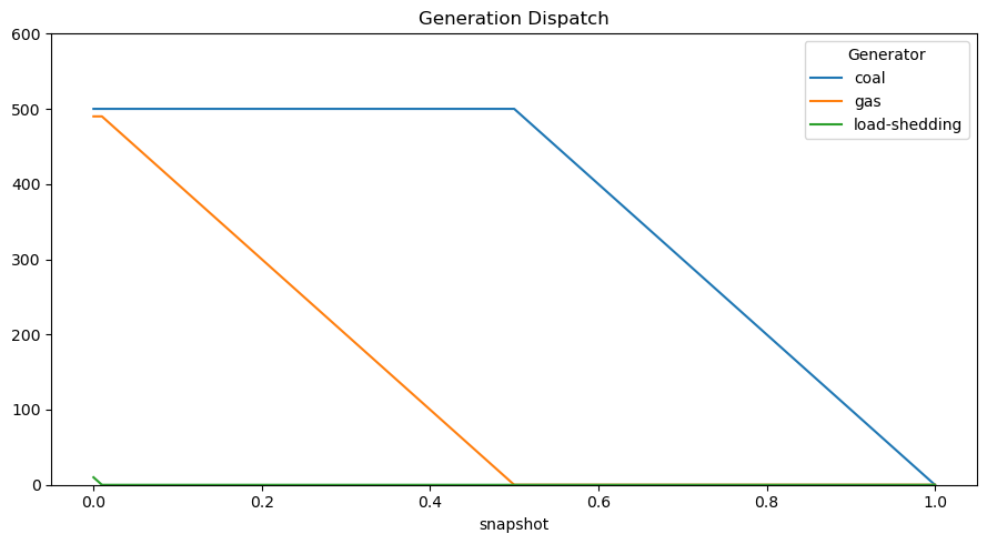
../_images/examples_generation-investment-screening-curve_14_0.png

Demonstrate zero-profit condition.

The total cost is given by

[11]:

(
    n.generators.p_nom_opt * n.generators.capital_cost
    + n.generators_t.p.multiply(n.snapshot_weightings.generators, axis=0).sum()
    * n.generators.marginal_cost
)

[11]:

Generator
coal             8249.750250
gas              6400.839161
load-shedding      55.604396
dtype: float64

The total revenue by

[12]:

(
    n.generators_t.p.multiply(n.snapshot_weightings.generators, axis=0)
    .multiply(n.buses_t.marginal_price["bus"], axis=0)
    .sum(0)
)

[12]:

Generator
coal             8249.750198
gas              6400.839108
load-shedding      55.604395
dtype: float64

Now, take the capacities from the above long-term equilibrium, then disallow expansion.

Show that the resulting market prices are identical.

This holds in this example, but does NOT necessarily hold and breaks down in some circumstances (for example, when there is a lot of storage and inter-temporal shifting).

[13]:

n.generators.p_nom_extendable = False
n.generators.p_nom = n.generators.p_nom_opt

[14]:

n.optimize();

INFO:linopy.model: Solve problem using Glpk solver

INFO:linopy.io: Writing time: 0.05s

INFO:linopy.solvers:GLPSOL--GLPK LP/MIP Solver 5.0
Parameter(s) specified in the command line:
 --lp /tmp/linopy-problem-msciqexw.lp --output /tmp/linopy-solve-yq1fg8e6.sol
Reading problem data from '/tmp/linopy-problem-msciqexw.lp'...
7007 rows, 3003 columns, 9009 non-zeros
36046 lines were read
GLPK Simplex Optimizer 5.0
7007 rows, 3003 columns, 9009 non-zeros
Preprocessing...
998 rows, 1996 columns, 1996 non-zeros
Scaling...
 A: min|aij| =  1.000e+00  max|aij| =  1.000e+00  ratio =  1.000e+00
Problem data seem to be well scaled
Constructing initial basis...
Size of triangular part is 998
      0: obj =   1.014985015e+03 inf =   1.248e+05 (499)
    508: obj =   2.306193806e+03 inf =   0.000e+00 (0)
*   509: obj =   2.306193806e+03 inf =   0.000e+00 (0)
OPTIMAL LP SOLUTION FOUND
Time used:   0.0 secs
Memory used: 4.4 Mb (4648204 bytes)
Writing basic solution to '/tmp/linopy-solve-yq1fg8e6.sol'...

INFO:linopy.constants: Optimization successful:
Status: ok
Termination condition: optimal
Solution: 3003 primals, 7007 duals
Objective: 2.31e+03
Solver model: not available
Solver message: optimal

INFO:pypsa.optimization.optimize:The shadow-prices of the constraints Generator-fix-p-lower, Generator-fix-p-upper were not assigned to the network.

[15]:

n.buses_t.marginal_price.plot(title="Price Duration Curve", figsize=(9, 5))
plt.tight_layout()

../_images/examples_generation-investment-screening-curve_22_0.png

[16]:

n.buses_t.marginal_price.sum(axis=1).value_counts()

[16]:

1.999998       500
11.999988      490
1012.000990     10
0.000000         1
Name: count, dtype: int64

Demonstrate zero-profit condition. Differences are due to singular times, see above, not a problem

Total costs

[17]:

(
    n.generators.p_nom * n.generators.capital_cost
    + n.generators_t.p.multiply(n.snapshot_weightings.generators, axis=0).sum()
    * n.generators.marginal_cost
)

[17]:

Generator
coal             8249.750250
gas              6400.839161
load-shedding      55.604396
dtype: float64

Total revenue

[18]:

(
    n.generators_t.p.multiply(n.snapshot_weightings.generators, axis=0)
    .multiply(n.buses_t.marginal_price["bus"], axis=0)
    .sum()
)

[18]:

Generator
coal             8242.25950
gas              6395.94746
load-shedding      55.60445
dtype: float64