Note
You can download this example as a Jupyter notebook or start it in interactive mode.
Redispatch Example with SciGRID network#
In this example, we compare a 2-stage market with an initial market clearing in two bidding zones with flow-based market coupling and a subsequent redispatch market (incl. curtailment) to an idealised nodal pricing scheme.
[1]:
import pypsa
import matplotlib.pyplot as plt
import cartopy.crs as ccrs
from pypsa.descriptors import get_switchable_as_dense as as_dense
ERROR 1: PROJ: proj_create_from_database: Open of /home/docs/checkouts/readthedocs.org/user_builds/pypsa/conda/latest/share/proj failed
[2]:
solver = "cbc"
Load example network#
[3]:
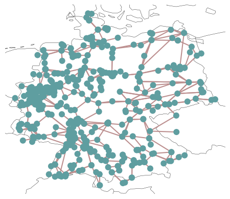
o = pypsa.examples.scigrid_de(from_master=True)
o.lines.s_max_pu = 0.7
o.lines.loc[["316", "527", "602"], "s_nom"] = 1715
o.set_snapshots([o.snapshots[12]])
WARNING:pypsa.io:Importing network from PyPSA version v0.17.1 while current version is v0.27.1. Read the release notes at https://pypsa.readthedocs.io/en/latest/release_notes.html to prepare your network for import.
INFO:pypsa.io:Imported network scigrid-de.nc has buses, generators, lines, loads, storage_units, transformers
[4]:
n = o.copy()  # for redispatch model
m = o.copy()  # for market model
[5]:
o.plot();
/home/docs/checkouts/readthedocs.org/user_builds/pypsa/conda/latest/lib/python3.11/site-packages/cartopy/mpl/feature_artist.py:144: UserWarning: facecolor will have no effect as it has been defined as "never".
  warnings.warn('facecolor will have no effect as it has been '
Solve original nodal market model o#
First, let us solve a nodal market using the original model o:
[6]:
o.optimize(solver_name=solver)
WARNING:pypsa.components:The following transformers have zero r, which could break the linear load flow:
Index(['2', '5', '10', '12', '13', '15', '18', '20', '22', '24', '26', '30',
       '32', '37', '42', '46', '52', '56', '61', '68', '69', '74', '78', '86',
       '87', '94', '95', '96', '99', '100', '104', '105', '106', '107', '117',
       '120', '123', '124', '125', '128', '129', '138', '143', '156', '157',
       '159', '160', '165', '184', '191', '195', '201', '220', '231', '232',
       '233', '236', '247', '248', '250', '251', '252', '261', '263', '264',
       '267', '272', '279', '281', '282', '292', '303', '307', '308', '312',
       '315', '317', '322', '332', '334', '336', '338', '351', '353', '360',
       '362', '382', '384', '385', '391', '403', '404', '413', '421', '450',
       '458'],
      dtype='object', name='Transformer')
INFO:linopy.model: Solve problem using Cbc solver
INFO:linopy.io: Writing time: 0.1s
INFO:linopy.solvers:Welcome to the CBC MILP Solver
Version: 2.10.10
Build Date: Apr 19 2023

command line - cbc -printingOptions all -import /tmp/linopy-problem-mw1shgzf.lp -solve -solu /tmp/linopy-solve-_d4prguh.sol (default strategy 1)
Option for printingOptions changed from normal to all
Presolve 629 (-5328) rows, 1091 (-1394) columns and 3871 (-7077) elements
Perturbing problem by 0.001% of 2769.2736 - largest nonzero change 0.00099220524 ( 0.0061979697%) - largest zero change 0.00098939989
0  Obj -9.5083027 Primal inf 1298365.2 (581)
87  Obj -9.2453851 Primal inf 736836.08 (538)
174  Obj -9.1687351 Primal inf 885985.69 (529)
232  Obj -8.9230987 Primal inf 890466.24 (502)
300  Obj -7.9224648 Primal inf 643744.18 (467)
371  Obj -5.8404701 Primal inf 731238.9 (429)
444  Obj 3998.1369 Primal inf 777939.54 (327)
507  Obj 4000.1194 Primal inf 1823422.9 (359)
580  Obj 4389.4002 Primal inf 808502.75 (233)
659  Obj 151151.3 Primal inf 14901.518 (87)
746  Obj 297651.07 Primal inf 22921.947 (99)
773  Obj 301211.09
Optimal - objective value 301209.38
After Postsolve, objective 301209.38, infeasibilities - dual 0 (0), primal 0 (0)
Optimal objective 301209.3823 - 773 iterations time 0.122, Presolve 0.02
Total time (CPU seconds):       0.20   (Wallclock seconds):       0.11
INFO:linopy.constants: Optimization successful:
Status: ok
Termination condition: optimal
Solution: 2485 primals, 5957 duals
Objective: 3.01e+05
Solver model: not available
Solver message: Optimal - objective value 301209.38232509
INFO:pypsa.optimization.optimize:The shadow-prices of the constraints Generator-fix-p-lower, Generator-fix-p-upper, Line-fix-s-lower, Line-fix-s-upper, Transformer-fix-s-lower, Transformer-fix-s-upper, StorageUnit-fix-p_dispatch-lower, StorageUnit-fix-p_dispatch-upper, StorageUnit-fix-p_store-lower, StorageUnit-fix-p_store-upper, StorageUnit-fix-state_of_charge-lower, StorageUnit-fix-state_of_charge-upper, Kirchhoff-Voltage-Law, StorageUnit-energy_balance were not assigned to the network.
[6]:
('ok', 'optimal')
Costs are 301 k€.
Build market model m with two bidding zones#
For this example, we split the German transmission network into two market zones at latitude 51 degrees.
You can build any other market zones by providing an alternative mapping from bus to zone.
[7]:
zones = (n.buses.y > 51).map(lambda x: "North" if x else "South")
Next, we assign this mapping to the market model m.
We re-assign the buses of all generators and loads, and remove all transmission lines within each bidding zone.
Here, we assume that the bidding zones are coupled through the transmission lines that connect them.
[8]:
for c in m.iterate_components(m.one_port_components):
    c.df.bus = c.df.bus.map(zones)

for c in m.iterate_components(m.branch_components):
    c.df.bus0 = c.df.bus0.map(zones)
    c.df.bus1 = c.df.bus1.map(zones)
    internal = c.df.bus0 == c.df.bus1
    m.mremove(c.name, c.df.loc[internal].index)

m.mremove("Bus", m.buses.index)
m.madd("Bus", ["North", "South"]);
Now, we can solve the coupled market with two bidding zones.
[9]:
m.optimize(solver_name=solver)
INFO:linopy.model: Solve problem using Cbc solver
INFO:linopy.io: Writing time: 0.07s
INFO:linopy.solvers:Welcome to the CBC MILP Solver
Version: 2.10.10
Build Date: Apr 19 2023

command line - cbc -printingOptions all -import /tmp/linopy-problem-mzxwpuwr.lp -solve -solu /tmp/linopy-solve-87iiix0b.sol (default strategy 1)
Option for printingOptions changed from normal to all
Presolve 40 (-3145) rows, 410 (-1151) columns and 487 (-4342) elements
Perturbing problem by 0.001% of 212.59539 - largest nonzero change 0.00017578427 ( 0.0036987348%) - largest zero change 0.00015445146
0  Obj 0 Primal inf 11285.222 (1)
48  Obj 184184.9 Primal inf 1700.1029 (24)
86  Obj 213988.73
Optimal - objective value 213988.69
After Postsolve, objective 213988.69, infeasibilities - dual 0 (0), primal 0 (0)
Optimal objective 213988.686 - 86 iterations time 0.012, Presolve 0.01
Total time (CPU seconds):       0.05   (Wallclock seconds):       0.03
INFO:linopy.constants: Optimization successful:
Status: ok
Termination condition: optimal
Solution: 1561 primals, 3185 duals
Objective: 2.14e+05
Solver model: not available
Solver message: Optimal - objective value 213988.68595810
INFO:pypsa.optimization.optimize:The shadow-prices of the constraints Generator-fix-p-lower, Generator-fix-p-upper, Line-fix-s-lower, Line-fix-s-upper, StorageUnit-fix-p_dispatch-lower, StorageUnit-fix-p_dispatch-upper, StorageUnit-fix-p_store-lower, StorageUnit-fix-p_store-upper, StorageUnit-fix-state_of_charge-lower, StorageUnit-fix-state_of_charge-upper, Kirchhoff-Voltage-Law, StorageUnit-energy_balance were not assigned to the network.
[9]:
('ok', 'optimal')
Costs are 214 k€, which is much lower than the 301 k€ of the nodal market.
This is because network restrictions apart from the North/South division are not taken into account yet.
We can look at the market clearing prices of each zone:
[10]:
m.buses_t.marginal_price
[10]:
| Bus | North | South |
|---|---|---|
| snapshot | ||
| 2011-01-01 12:00:00 | 8.0 | 25.0 |
Build redispatch model n#
Next, based on the market outcome with two bidding zones m, we build a secondary redispatch market n that rectifies transmission constraints through curtailment and ramping up/down thermal generators.
First, we fix the dispatch of generators to the results from the market simulation. (For simplicity, this example disregards storage units.)
[11]:
p = m.generators_t.p / m.generators.p_nom
n.generators_t.p_min_pu = p
n.generators_t.p_max_pu = p
Then, we add generators bidding into redispatch market using the following assumptions:
All generators can reduce their dispatch to zero. This includes also curtailment of renewables.
All generators can increase their dispatch to their available/nominal capacity.
No changes to the marginal costs, i.e. reducing dispatch lowers costs.
With these settings, the 2-stage market should result in the same cost as the nodal market.
[12]:
g_up = n.generators.copy()
g_down = n.generators.copy()

g_up.index = g_up.index.map(lambda x: x + " ramp up")
g_down.index = g_down.index.map(lambda x: x + " ramp down")

up = (
    as_dense(m, "Generator", "p_max_pu") * m.generators.p_nom - m.generators_t.p
).clip(0) / m.generators.p_nom
down = -m.generators_t.p / m.generators.p_nom

up.columns = up.columns.map(lambda x: x + " ramp up")
down.columns = down.columns.map(lambda x: x + " ramp down")

n.madd("Generator", g_up.index, p_max_pu=up, **g_up.drop("p_max_pu", axis=1))

n.madd(
    "Generator",
    g_down.index,
    p_min_pu=down,
    p_max_pu=0,
    **g_down.drop(["p_max_pu", "p_min_pu"], axis=1)
);
Now, let’s solve the redispatch market:
[13]:
n.optimize(solver_name=solver)
WARNING:pypsa.components:The following transformers have zero r, which could break the linear load flow:
Index(['2', '5', '10', '12', '13', '15', '18', '20', '22', '24', '26', '30',
       '32', '37', '42', '46', '52', '56', '61', '68', '69', '74', '78', '86',
       '87', '94', '95', '96', '99', '100', '104', '105', '106', '107', '117',
       '120', '123', '124', '125', '128', '129', '138', '143', '156', '157',
       '159', '160', '165', '184', '191', '195', '201', '220', '231', '232',
       '233', '236', '247', '248', '250', '251', '252', '261', '263', '264',
       '267', '272', '279', '281', '282', '292', '303', '307', '308', '312',
       '315', '317', '322', '332', '334', '336', '338', '351', '353', '360',
       '362', '382', '384', '385', '391', '403', '404', '413', '421', '450',
       '458'],
      dtype='object', name='Transformer')
INFO:linopy.model: Solve problem using Cbc solver
INFO:linopy.io: Writing time: 0.13s
INFO:linopy.solvers:Welcome to the CBC MILP Solver
Version: 2.10.10
Build Date: Apr 19 2023

command line - cbc -printingOptions all -import /tmp/linopy-problem-yo3jyq1d.lp -solve -solu /tmp/linopy-solve-66s46ul8.sol (default strategy 1)
Option for printingOptions changed from normal to all
Presolve 633 (-11016) rows, 1310 (-4021) columns and 4103 (-15383) elements
Perturbing problem by 0.001% of 2769.2736 - largest nonzero change 0.00099112912 ( 0.0086739515%) - largest zero change 0.00099083499
0  Obj 195157.16 Primal inf 1314652.2 (583) Dual inf 9200.1216 (158)
87  Obj -9.6713575 Primal inf 769507.01 (549)
174  Obj -9.3082844 Primal inf 1180847.3 (523)
259  Obj -8.3881407 Primal inf 2384207.8 (471)
335  Obj -6.9770532 Primal inf 686901.11 (444)
400  Obj -5.9197761 Primal inf 405527.04 (364)
463  Obj 3997.9253 Primal inf 2037328.8 (418)
538  Obj 4000.0346 Primal inf 1411433.8 (321)
625  Obj 4034.2482 Primal inf 2462659.5 (325)
706  Obj 80535.292 Primal inf 20404296 (294)
793  Obj 211492.65 Primal inf 32617.407 (98)
876  Obj 301210.93
876  Obj 301209.38 Dual inf 1.4139822e-05 (3)
879  Obj 301209.38
Optimal - objective value 301209.38
After Postsolve, objective 301209.38, infeasibilities - dual 1520.3083 (101), primal 2.2809491e-05 (95)
Presolved model was optimal, full model needs cleaning up
0  Obj 301209.38 Primal inf 1.9906078e-07 (2) Dual inf 2.0000001e+08 (103)
End of values pass after 105 iterations
105  Obj 301209.38
Optimal - objective value 301209.38
Optimal objective 301209.3811 - 984 iterations time 0.162, Presolve 0.03
Total time (CPU seconds):       0.26   (Wallclock seconds):       0.16
INFO:linopy.constants: Optimization successful:
Status: ok
Termination condition: optimal
Solution: 5331 primals, 11649 duals
Objective: 3.01e+05
Solver model: not available
Solver message: Optimal - objective value 301209.38114435
INFO:pypsa.optimization.optimize:The shadow-prices of the constraints Generator-fix-p-lower, Generator-fix-p-upper, Line-fix-s-lower, Line-fix-s-upper, Transformer-fix-s-lower, Transformer-fix-s-upper, StorageUnit-fix-p_dispatch-lower, StorageUnit-fix-p_dispatch-upper, StorageUnit-fix-p_store-lower, StorageUnit-fix-p_store-upper, StorageUnit-fix-state_of_charge-lower, StorageUnit-fix-state_of_charge-upper, Kirchhoff-Voltage-Law, StorageUnit-energy_balance were not assigned to the network.
[13]:
('ok', 'optimal')
And, as expected, the costs are the same as for the nodal market: 301 k€.
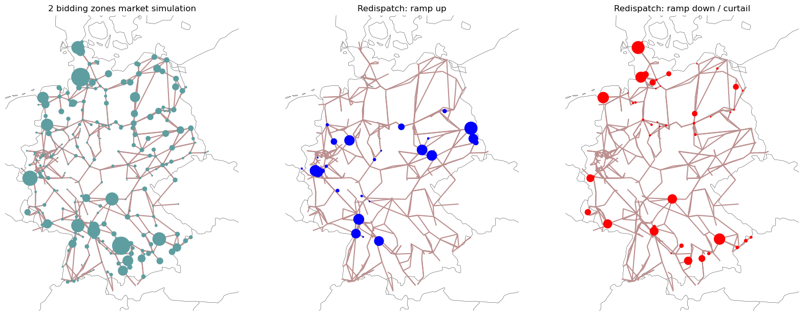
Now, we can plot both the market results of the 2 bidding zone market and the redispatch results:
[14]:
fig, axs = plt.subplots(
    1, 3, figsize=(20, 10), subplot_kw={"projection": ccrs.AlbersEqualArea()}
)

market = (
    n.generators_t.p[m.generators.index]
    .T.squeeze()
    .groupby(n.generators.bus)
    .sum()
    .div(2e4)
)
n.plot(ax=axs[0], bus_sizes=market, title="2 bidding zones market simulation")

redispatch_up = (
    n.generators_t.p.filter(like="ramp up")
    .T.squeeze()
    .groupby(n.generators.bus)
    .sum()
    .div(2e4)
)
n.plot(
    ax=axs[1], bus_sizes=redispatch_up, bus_colors="blue", title="Redispatch: ramp up"
)

redispatch_down = (
    n.generators_t.p.filter(like="ramp down")
    .T.squeeze()
    .groupby(n.generators.bus)
    .sum()
    .div(-2e4)
)
n.plot(
    ax=axs[2],
    bus_sizes=redispatch_down,
    bus_colors="red",
    title="Redispatch: ramp down / curtail",
);
/home/docs/checkouts/readthedocs.org/user_builds/pypsa/conda/latest/lib/python3.11/site-packages/cartopy/mpl/feature_artist.py:144: UserWarning: facecolor will have no effect as it has been defined as "never".
  warnings.warn('facecolor will have no effect as it has been '
/home/docs/checkouts/readthedocs.org/user_builds/pypsa/conda/latest/lib/python3.11/site-packages/cartopy/mpl/feature_artist.py:144: UserWarning: facecolor will have no effect as it has been defined as "never".
  warnings.warn('facecolor will have no effect as it has been '
/home/docs/checkouts/readthedocs.org/user_builds/pypsa/conda/latest/lib/python3.11/site-packages/cartopy/mpl/feature_artist.py:144: UserWarning: facecolor will have no effect as it has been defined as "never".
  warnings.warn('facecolor will have no effect as it has been '
We can also read out the final dispatch of each generator:
[15]:
grouper = n.generators.index.str.split(" ramp", expand=True).get_level_values(0)

n.generators_t.p.groupby(grouper, axis=1).sum().squeeze()
/tmp/ipykernel_4996/2204001103.py:3: FutureWarning: DataFrame.groupby with axis=1 is deprecated. Do `frame.T.groupby(...)` without axis instead.
  n.generators_t.p.groupby(grouper, axis=1).sum().squeeze()
[15]:
1 Gas                     0.000000
1 Hard Coal               0.000000
1 Solar                  11.326192
1 Wind Onshore            1.754375
100_220kV Solar          14.913326
                           ...
98 Wind Onshore          71.451646
99_220kV Gas              0.000000
99_220kV Hard Coal        0.000000
99_220kV Solar            8.246606
99_220kV Wind Onshore     3.432939
Name: 2011-01-01 12:00:00, Length: 1423, dtype: float64
Changing bidding strategies in redispatch market#
We can also formulate other bidding strategies or compensation mechanisms for the redispatch market.
For example, that ramping up a generator is twice as expensive.
[16]:
n.generators.loc[n.generators.index.str.contains("ramp up"), "marginal_cost"] *= 2
Or that generators need to be compensated for curtailing them or ramping them down at 50% of their marginal cost.
[17]:
n.generators.loc[n.generators.index.str.contains("ramp down"), "marginal_cost"] *= -0.5
In this way, the outcome should be more expensive than the ideal nodal market:
[18]:
n.optimize(solver_name=solver)
WARNING:pypsa.components:The following transformers have zero r, which could break the linear load flow:
Index(['2', '5', '10', '12', '13', '15', '18', '20', '22', '24', '26', '30',
       '32', '37', '42', '46', '52', '56', '61', '68', '69', '74', '78', '86',
       '87', '94', '95', '96', '99', '100', '104', '105', '106', '107', '117',
       '120', '123', '124', '125', '128', '129', '138', '143', '156', '157',
       '159', '160', '165', '184', '191', '195', '201', '220', '231', '232',
       '233', '236', '247', '248', '250', '251', '252', '261', '263', '264',
       '267', '272', '279', '281', '282', '292', '303', '307', '308', '312',
       '315', '317', '322', '332', '334', '336', '338', '351', '353', '360',
       '362', '382', '384', '385', '391', '403', '404', '413', '421', '450',
       '458'],
      dtype='object', name='Transformer')
WARNING:pypsa.components:The following transformers have zero r, which could break the linear load flow:
Index(['2', '5', '10', '12', '13', '15', '18', '20', '22', '24', '26', '30',
       '32', '37', '42', '46', '52', '56', '61', '68', '69', '74', '78', '86',
       '87', '94', '95', '96', '99', '100', '104', '105', '106', '107', '117',
       '120', '123', '124', '125', '128', '129', '138', '143', '156', '157',
       '159', '160', '165', '184', '191', '195', '201', '220', '231', '232',
       '233', '236', '247', '248', '250', '251', '252', '261', '263', '264',
       '267', '272', '279', '281', '282', '292', '303', '307', '308', '312',
       '315', '317', '322', '332', '334', '336', '338', '351', '353', '360',
       '362', '382', '384', '385', '391', '403', '404', '413', '421', '450',
       '458'],
      dtype='object', name='Transformer')
INFO:linopy.model: Solve problem using Cbc solver
INFO:linopy.io: Writing time: 0.13s
INFO:linopy.solvers:Welcome to the CBC MILP Solver
Version: 2.10.10
Build Date: Apr 19 2023

command line - cbc -printingOptions all -import /tmp/linopy-problem-9xs65bdw.lp -solve -solu /tmp/linopy-solve-y7mnqixe.sol (default strategy 1)
Option for printingOptions changed from normal to all
Presolve 633 (-11016) rows, 1311 (-4020) columns and 4104 (-15382) elements
Perturbing problem by 0.001% of 5538.5472 - largest nonzero change 0.00089645788 ( 0.0019742048%) - largest zero change 0.00087218034
0  Obj 223388.71 Primal inf 1314652.2 (583)
87  Obj 223388.93 Primal inf 795599.81 (549)
174  Obj 223389.29 Primal inf 1051716.4 (518)
254  Obj 223391.16 Primal inf 624464.87 (473)
341  Obj 223392.53 Primal inf 409927.53 (420)
426  Obj 230850.37 Primal inf 1916178.4 (386)
506  Obj 230853.16 Primal inf 2455720.3 (284)
579  Obj 230856.9 Primal inf 338721.66 (227)
657  Obj 231735.96 Primal inf 195832.48 (159)
744  Obj 329611.98 Primal inf 61391.074 (62) Dual inf 3.5480093e-18 (1)
814  Obj 479005.11
814  Obj 479003.13 Dual inf 0.00051466733 (19)
823  Obj 479003.12
Optimal - objective value 479003.12
After Postsolve, objective 479003.12, infeasibilities - dual 2802.1431 (91), primal 1.9618797e-05 (84)
Presolved model was optimal, full model needs cleaning up
0  Obj 479003.12 Primal inf 2.8680472e-07 (2) Dual inf 2.0000003e+08 (93)
End of values pass after 94 iterations
94  Obj 479003.12
Optimal - objective value 479003.12
Optimal objective 479003.1219 - 917 iterations time 0.142, Presolve 0.03
Total time (CPU seconds):       0.24   (Wallclock seconds):       0.15
INFO:linopy.constants: Optimization successful:
Status: ok
Termination condition: optimal
Solution: 5331 primals, 11649 duals
Objective: 4.79e+05
Solver model: not available
Solver message: Optimal - objective value 479003.12190570
INFO:pypsa.optimization.optimize:The shadow-prices of the constraints Generator-fix-p-lower, Generator-fix-p-upper, Line-fix-s-lower, Line-fix-s-upper, Transformer-fix-s-lower, Transformer-fix-s-upper, StorageUnit-fix-p_dispatch-lower, StorageUnit-fix-p_dispatch-upper, StorageUnit-fix-p_store-lower, StorageUnit-fix-p_store-upper, StorageUnit-fix-state_of_charge-lower, StorageUnit-fix-state_of_charge-upper, Kirchhoff-Voltage-Law, StorageUnit-energy_balance were not assigned to the network.
[18]:
('ok', 'optimal')
Costs are now 502 k€ compared to 301 k€.