Note
You can download this example as a Jupyter notebook or start it in interactive mode.
Using the statistics module in PyPSA#
The statistics module is used to easily extract information from your networks. This is useful when inspecting your solved networks and creating first visualizations of your results.
With the statistics module, you can look at different metrics of your network. A list of the implemented metrics are:
Capital expenditure
Operational expenditure
Installed capacities
Optimal capacities
Supply
Withdrawal
Curtailment
Capacity Factor
Revenue
Market value
Energy balance
Now lets look at an example.
[1]:
import pypsa
import matplotlib.pyplot as plt
import numpy as np
ERROR 1: PROJ: proj_create_from_database: Open of /home/docs/checkouts/readthedocs.org/user_builds/pypsa/conda/stable/share/proj failed
First, we open an example network we want to investigate.
[2]:
n = pypsa.examples.scigrid_de()
WARNING:pypsa.io:Importing network from PyPSA version v0.17.1 while current version is v0.27.1. Read the release notes at https://pypsa.readthedocs.io/en/latest/release_notes.html to prepare your network for import.
INFO:pypsa.io:Imported network scigrid-de.nc has buses, generators, lines, loads, storage_units, transformers
Lets run an overview of all statistics by calling:
[3]:
n.statistics().dropna()
[3]:
| Optimal Capacity | Installed Capacity | Capacity Factor | Dispatch | Transmission | Withdrawal | Supply | Curtailment | Capital Expenditure | Operational Expenditure | Revenue | Market Value | ||
|---|---|---|---|---|---|---|---|---|---|---|---|---|---|
| Generator | Brown Coal | 0.0 | 20879.500000 | 0.0 | 0.0 | 0.0 | 0.0 | 0.0 | 0.0 | 0.0 | 0.0 | 0.0 | 0.0 |
| Gas | 0.0 | 23913.130000 | 0.0 | 0.0 | 0.0 | 0.0 | 0.0 | 0.0 | 0.0 | 0.0 | 0.0 | 0.0 | |
| Geothermal | 0.0 | 31.700000 | 0.0 | 0.0 | 0.0 | 0.0 | 0.0 | 0.0 | 0.0 | 0.0 | 0.0 | 0.0 | |
| Hard Coal | 0.0 | 25312.600000 | 0.0 | 0.0 | 0.0 | 0.0 | 0.0 | 0.0 | 0.0 | 0.0 | 0.0 | 0.0 | |
| Multiple | 0.0 | 152.700000 | 0.0 | 0.0 | 0.0 | 0.0 | 0.0 | 0.0 | 0.0 | 0.0 | 0.0 | 0.0 | |
| Nuclear | 0.0 | 12068.000000 | 0.0 | 0.0 | 0.0 | 0.0 | 0.0 | 0.0 | 0.0 | 0.0 | 0.0 | 0.0 | |
| Oil | 0.0 | 2710.200000 | 0.0 | 0.0 | 0.0 | 0.0 | 0.0 | 0.0 | 0.0 | 0.0 | 0.0 | 0.0 | |
| Other | 0.0 | 3027.800000 | 0.0 | 0.0 | 0.0 | 0.0 | 0.0 | 0.0 | 0.0 | 0.0 | 0.0 | 0.0 | |
| Run of River | 0.0 | 3999.100000 | 0.0 | 0.0 | 0.0 | 0.0 | 0.0 | 0.0 | 0.0 | 0.0 | 0.0 | 0.0 | |
| Solar | 0.0 | 37041.524779 | 0.0 | 0.0 | 0.0 | 0.0 | 0.0 | 0.0 | 0.0 | 0.0 | 0.0 | 0.0 | |
| Storage Hydro | 0.0 | 1445.000000 | 0.0 | 0.0 | 0.0 | 0.0 | 0.0 | 0.0 | 0.0 | 0.0 | 0.0 | 0.0 | |
| Waste | 0.0 | 1645.900000 | 0.0 | 0.0 | 0.0 | 0.0 | 0.0 | 0.0 | 0.0 | 0.0 | 0.0 | 0.0 | |
| Wind Offshore | 0.0 | 2973.500000 | 0.0 | 0.0 | 0.0 | 0.0 | 0.0 | 0.0 | 0.0 | 0.0 | 0.0 | 0.0 | |
| Wind Onshore | 0.0 | 37339.895329 | 0.0 | 0.0 | 0.0 | 0.0 | 0.0 | 0.0 | 0.0 | 0.0 | 0.0 | 0.0 | |
| Line | - | 0.0 | 961101.136714 | 0.0 | 0.0 | 0.0 | 0.0 | 0.0 | 0.0 | 0.0 | 0.0 | 0.0 | 0.0 |
| StorageUnit | Pumped Hydro | 0.0 | 9179.500000 | 0.0 | 0.0 | 0.0 | 0.0 | 0.0 | 0.0 | 0.0 | 0.0 | 0.0 | 0.0 |
| Transformer | - | 0.0 | 192000.000000 | 0.0 | 0.0 | 0.0 | 0.0 | 0.0 | 0.0 | 0.0 | 0.0 | 0.0 | 0.0 |
So far the statistics are not so interesting, because we have not solved the network yet. We can only see that the network already has some installed capacities for different components.
You can see that statistics returns a pandas.DataFrame. The MultiIndex of the DataFrame provides the name of the network component (i.e. first entry of the MultiIndex, like Generator, Line,…) on the first index level. The carrier index level provides the carrier name of the given component. For example, in n.generators, we have the carriers Brown Coal, Gas and so on.
Now lets solve the network.
[4]:
n.optimize(n.snapshots[:4])
WARNING:pypsa.components:The following transformers have zero r, which could break the linear load flow:
Index(['2', '5', '10', '12', '13', '15', '18', '20', '22', '24', '26', '30',
       '32', '37', '42', '46', '52', '56', '61', '68', '69', '74', '78', '86',
       '87', '94', '95', '96', '99', '100', '104', '105', '106', '107', '117',
       '120', '123', '124', '125', '128', '129', '138', '143', '156', '157',
       '159', '160', '165', '184', '191', '195', '201', '220', '231', '232',
       '233', '236', '247', '248', '250', '251', '252', '261', '263', '264',
       '267', '272', '279', '281', '282', '292', '303', '307', '308', '312',
       '315', '317', '322', '332', '334', '336', '338', '351', '353', '360',
       '362', '382', '384', '385', '391', '403', '404', '413', '421', '450',
       '458'],
      dtype='object', name='Transformer')
INFO:linopy.model: Solve problem using Glpk solver
INFO:linopy.io: Writing time: 0.18s
INFO:linopy.solvers:GLPSOL--GLPK LP/MIP Solver 5.0
Parameter(s) specified in the command line:
 --lp /tmp/linopy-problem-rw60edon.lp --output /tmp/linopy-solve-jtoaa2y_.sol
Reading problem data from '/tmp/linopy-problem-rw60edon.lp'...
23828 rows, 9940 columns, 43518 non-zeros
126856 lines were read
GLPK Simplex Optimizer 5.0
23828 rows, 9940 columns, 43518 non-zeros
Preprocessing...
3772 rows, 5708 columns, 19230 non-zeros
Scaling...
 A: min|aij| =  1.485e-02  max|aij| =  1.974e+02  ratio =  1.329e+04
GM: min|aij| =  1.907e-01  max|aij| =  5.245e+00  ratio =  2.751e+01
EQ: min|aij| =  3.652e-02  max|aij| =  1.000e+00  ratio =  2.738e+01
Constructing initial basis...
Size of triangular part is 3669
      0: obj =   1.220672167e+08 inf =   5.882e+07 (2919)
   6953: obj =   4.298431274e+06 inf =   6.810e-11 (0) 41
*  9382: obj =   1.038959807e+06 inf =   0.000e+00 (0) 8
OPTIMAL LP SOLUTION FOUND
Time used:   2.1 secs
Memory used: 17.2 Mb (18047092 bytes)
Writing basic solution to '/tmp/linopy-solve-jtoaa2y_.sol'...
INFO:linopy.constants: Optimization successful:
Status: ok
Termination condition: optimal
Solution: 9940 primals, 23828 duals
Objective: 1.04e+06
Solver model: not available
Solver message: optimal
INFO:pypsa.optimization.optimize:The shadow-prices of the constraints Generator-fix-p-lower, Generator-fix-p-upper, Line-fix-s-lower, Line-fix-s-upper, Transformer-fix-s-lower, Transformer-fix-s-upper, StorageUnit-fix-p_dispatch-lower, StorageUnit-fix-p_dispatch-upper, StorageUnit-fix-p_store-lower, StorageUnit-fix-p_store-upper, StorageUnit-fix-state_of_charge-lower, StorageUnit-fix-state_of_charge-upper, Kirchhoff-Voltage-Law, StorageUnit-energy_balance were not assigned to the network.
[4]:
('ok', 'optimal')
Now we can look at the statistics of the solved network.
[5]:
n.statistics().round(1)
[5]:
| Optimal Capacity | Installed Capacity | Capacity Factor | Dispatch | Transmission | Withdrawal | Supply | Curtailment | Capital Expenditure | Operational Expenditure | Revenue | Market Value | ||
|---|---|---|---|---|---|---|---|---|---|---|---|---|---|
| Generator | Brown Coal | 20879.5 | 20879.5 | 0.1 | 42859.0 | 0.0 | 0.0 | 42859.0 | 0.0 | 0.0 | 428590.3 | 588266.5 | 13.7 |
| Gas | 23913.1 | 23913.1 | 0.0 | 79.4 | 0.0 | 0.0 | 79.4 | 0.0 | 0.0 | 3971.9 | 3971.9 | 50.0 | |
| Geothermal | 31.7 | 31.7 | 0.0 | 0.0 | 0.0 | 0.0 | 0.0 | 0.0 | 0.0 | 0.0 | 0.0 | 0.0 | |
| Hard Coal | 25312.6 | 25312.6 | 0.0 | 10535.7 | 0.0 | 0.0 | 10535.7 | 0.0 | 0.0 | 263391.6 | 272172.0 | 25.8 | |
| Multiple | 152.7 | 152.7 | 0.0 | 0.0 | 0.0 | 0.0 | 0.0 | 0.0 | 0.0 | 0.0 | 0.0 | 0.0 | |
| Nuclear | 12068.0 | 12068.0 | 0.1 | 31473.0 | 0.0 | 0.0 | 31473.0 | 0.0 | 0.0 | 251784.0 | 527108.2 | 16.7 | |
| Oil | 2710.2 | 2710.2 | 0.0 | 0.0 | 0.0 | 0.0 | 0.0 | 0.0 | 0.0 | 0.0 | 0.0 | 0.0 | |
| Other | 3027.8 | 3027.8 | 0.0 | 336.0 | 0.0 | 0.0 | 336.0 | 0.0 | 0.0 | 10752.0 | 11503.2 | 34.2 | |
| Run of River | 3999.1 | 3999.1 | 0.1 | 13723.3 | 0.0 | 0.0 | 13723.3 | 0.0 | 0.0 | 41170.0 | 301812.2 | 22.0 | |
| Solar | 37041.5 | 37041.5 | 0.0 | 0.0 | 0.0 | 0.0 | 0.0 | 47391.0 | 0.0 | 0.0 | 0.0 | 0.0 | |
| Storage Hydro | 1445.0 | 1445.0 | 0.1 | 3580.0 | 0.0 | 0.0 | 3580.0 | 0.0 | 0.0 | 10740.0 | 72904.4 | 20.4 | |
| Waste | 1645.9 | 1645.9 | 0.1 | 4760.0 | 0.0 | 0.0 | 4760.0 | 0.0 | 0.0 | 28560.0 | 97621.8 | 20.5 | |
| Wind Offshore | 2973.5 | 2973.5 | 0.1 | 7112.7 | 0.0 | 0.0 | 7112.7 | 62360.9 | 0.0 | 0.0 | 14034.2 | 2.0 | |
| Wind Onshore | 37339.9 | 37339.9 | 0.1 | 81882.7 | 0.0 | 0.0 | 81882.7 | 391557.6 | 0.0 | 0.0 | 406030.6 | 5.0 | |
| Line | AC | 961101.1 | 961101.1 | 0.0 | 0.0 | -17123.0 | 842901.4 | 842901.4 | 0.0 | 0.0 | 0.0 | 1045149.1 | 1.2 |
| Load | - | 0.0 | 0.0 | NaN | -195357.1 | 0.0 | 195357.1 | 0.0 | 0.0 | 0.0 | 0.0 | -3396077.6 | NaN |
| StorageUnit | Pumped Hydro | 9179.5 | 9179.5 | 0.0 | -984.7 | 0.0 | 984.7 | 0.0 | 0.0 | 0.0 | 0.0 | 4013.3 | NaN |
| Transformer | - | 192000.0 | 192000.0 | 0.0 | 0.0 | 14049.8 | 103460.9 | 103460.9 | 0.0 | 0.0 | 0.0 | 51490.2 | 0.5 |
As you can see there is now much more information available. There are still no capital expenditures in the network, because we only performed an operational optimization with this example network.
If you are interested in a specific metric, e.g. curtailment, you can run
[6]:
curtailment = n.statistics.curtailment()
curtailment[curtailment != 0]
[6]:
component  carrier
Generator  Solar             47391.043207
           Wind Offshore     62360.922344
           Wind Onshore     391557.618293
dtype: float64
Note that when calling a specific metric the statistics module returns a pandas.Series. To find the unit of the data returned by statistics, you can call attrs on the DataFrame or Series.
[7]:
curtailment.attrs
[7]:
{'name': 'Curtailment', 'unit': 'MWh'}
So the unit of curtailment is given in MWh. You can also customize your request.
For this you have various options: 1. You can select the component from which you want to get the metric with the attribute comps. Careful, comps has to be a list of strings.
[8]:
n.statistics.supply(comps=["Generator"])
[8]:
component  carrier
Generator  Brown Coal       42859.029000
           Gas                 79.437970
           Hard Coal        10535.663500
           Nuclear          31472.994000
           Other              336.000000
           Run of River     13723.318200
           Storage Hydro     3580.000000
           Waste             4760.000000
           Wind Offshore     7112.727000
           Wind Onshore     81882.665489
Name: generators, dtype: float64
For metrics which have a time dimension, you can choose the aggregation method or decide to not aggregate them at all. Just use the
aggregate_timeattribute to specify what you want to do.
For example calculate the mean supply/generation per time step is
[9]:
n.statistics.supply(comps=["Generator"], aggregate_time="mean")
[9]:
component  carrier
Generator  Brown Coal       1785.792875
           Gas                 3.309915
           Hard Coal         438.985979
           Nuclear          1311.374750
           Other              14.000000
           Run of River      571.804925
           Storage Hydro     149.166667
           Waste             198.333333
           Wind Offshore     296.363625
           Wind Onshore     3411.777729
Name: generators, dtype: float64
Or retrieve the supply time series by not aggregating the time series.
[10]:
n.statistics.supply(comps=["Generator"], aggregate_time=False).iloc[:, :4]
[10]:
| snapshot | 2011-01-01 00:00:00 | 2011-01-01 01:00:00 | 2011-01-01 02:00:00 | 2011-01-01 03:00:00 | |
|---|---|---|---|---|---|
| component | carrier | ||||
| Generator | Brown Coal | 12563.897000 | 10848.560000 | 10006.395000 | 9440.17700 |
| Gas | 35.826800 | 23.721700 | 13.083000 | 6.80647 | |
| Hard Coal | 4778.482000 | 3124.547000 | 1722.869000 | 909.76550 | |
| Nuclear | 7842.041000 | 7863.186000 | 7882.532000 | 7885.23500 | |
| Other | 84.000000 | 84.000000 | 84.000000 | 84.00000 | |
| Run of River | 3458.909000 | 3419.332800 | 3413.465800 | 3431.61060 | |
| Storage Hydro | 895.000000 | 895.000000 | 895.000000 | 895.00000 | |
| Waste | 1167.500000 | 1240.500000 | 1184.500000 | 1167.50000 | |
| Wind Offshore | 2489.407000 | 2217.742000 | 1039.115000 | 1366.46300 | |
| Wind Onshore | 18766.451072 | 20046.819368 | 21580.380209 | 21489.01484 |
You can choose how you want to group the components of the network and how to aggregate the groups. By default the components are grouped by their carriers and summed. However, you can change this by providing different
groupbyandaggregate_groupsattributes.
[11]:
n.statistics.supply(comps=["Generator"], groupby=["bus"], aggregate_groups="max")
[11]:
component  bus
Generator  101          1392.589000
           102           970.750000
           103             0.127076
           104_220kV       0.896977
           105_220kV      76.955900
                           ...
           94_220kV      164.614900
           95_220kV      186.429300
           96_220kV       53.032800
           97              0.002514
           98            335.603700
Name: generators, Length: 435, dtype: float64
Now you obtained the maximal supply in one time step for every bus in the network.
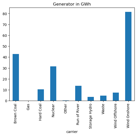
Often it is better when inspecting your network to visualize the tables. Therefore, you can easily make plots to analyze your results. For example the supply of the generators.
[12]:
n.statistics.supply(comps=["Generator"]).droplevel(0).div(1e3).plot.bar(
    title="Generator in GWh"
)
[12]:
<Axes: title={'center': 'Generator in GWh'}, xlabel='carrier'>
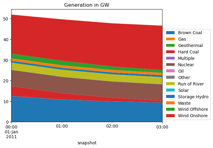
Or you could plot the generation time series of the generators.
[13]:
fig, ax = plt.subplots()
n.statistics.supply(comps=["Generator"], aggregate_time=False).droplevel(0).iloc[
    :, :4
].div(1e3).T.plot.area(
    title="Generation in GW",
    ax=ax,
    legend=False,
    linewidth=0,
)
ax.legend(bbox_to_anchor=(1, 0), loc="lower left", title=None, ncol=1)
[13]:
<matplotlib.legend.Legend at 0x7f7ce1a52e50>
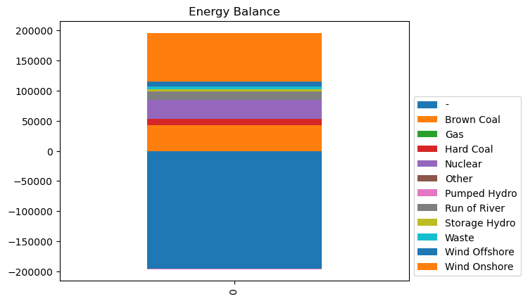
Finally, we want to look at the energy balance of the network. The energy balance is not included in the overview of the statistics module. To calculate the energy balance, you can do
[14]:
n.statistics.energy_balance()
[14]:
component    carrier        bus_carrier
Generator    Brown Coal     AC             4.285903e+04
             Gas            AC             7.943797e+01
             Geothermal     AC             0.000000e+00
             Hard Coal      AC             1.053566e+04
             Multiple       AC             0.000000e+00
             Nuclear        AC             3.147299e+04
             Oil            AC             0.000000e+00
             Other          AC             3.360000e+02
             Run of River   AC             1.372332e+04
             Solar          AC             0.000000e+00
             Storage Hydro  AC             3.580000e+03
             Waste          AC             4.760000e+03
             Wind Offshore  AC             7.112727e+03
             Wind Onshore   AC             8.188267e+04
Load         -              AC            -1.953571e+05
Transformer  -              AC             3.410605e-13
StorageUnit  Pumped Hydro   AC            -9.847483e+02
Line         AC             AC             1.136868e-12
dtype: float64
Note that there is now an additional index level called bus carrier. This is because an energy balance is defined for every bus carrier. The bus carriers you have in your network you can find by looking at n.buses.carrier.unique(). For this network, there is only one bus carrier which is AC and corresponds to electricity. However, you can have further bus carriers for example when you have a sector coupled network. You could have heat or CO \(_2\) as bus carrier. Therefore, for many
statistics functions you have to be careful about the units of the values and it is not always given by the attr object of the DataFrame or Series.
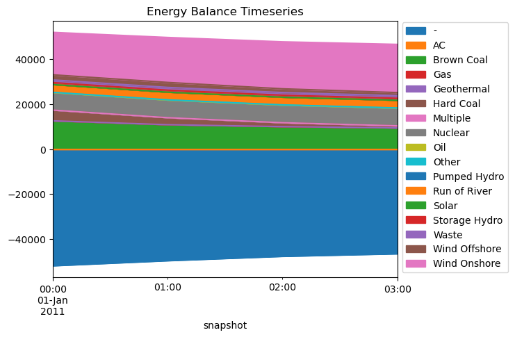
Finally, we want to plot the energy balance and the energy balance time series for electrcity which has the bus carrier AC. In a sector coupled network, you could also choose other bus carriers like H2 or heat. Note that in this example “-” represents the load in the system.
[15]:
fig, ax = plt.subplots()
n.statistics.energy_balance().loc[:, :, "AC"].groupby(
    "carrier"
).sum().to_frame().T.plot.bar(stacked=True, ax=ax, title="Energy Balance")
ax.legend(bbox_to_anchor=(1, 0), loc="lower left", title=None, ncol=1)
[15]:
<matplotlib.legend.Legend at 0x7f7d2401ba90>
[16]:
fig, ax = plt.subplots()
n.statistics.energy_balance(aggregate_time=False).loc[:, :, "AC"].droplevel(0).iloc[
    :, :4
].groupby("carrier").sum().where(lambda x: np.abs(x) > 1).fillna(0).T.plot.area(
    ax=ax, title="Energy Balance Timeseries"
)
ax.legend(bbox_to_anchor=(1, 0), loc="lower left", title=None, ncol=1)
[16]:
<matplotlib.legend.Legend at 0x7f7ce1aa4f10>