Note
You can download this example as a Jupyter notebook or start it in interactive mode.
Meshed AC-DC example
This example has a 3-node AC network coupled via AC-DC converters to a 3-node DC network. There is also a single point-to-point DC using the Link component.
The data files for this example are in the examples folder of the github repository: https://github.com/PyPSA/PyPSA.
[1]:
import pypsa
import numpy as np
import pandas as pd
import os
import matplotlib.pyplot as plt
import cartopy.crs as ccrs

%matplotlib inline
plt.rc("figure", figsize=(8, 8))
[2]:
network = pypsa.examples.ac_dc_meshed(from_master=True)
WARNING:pypsa.io:
Importing PyPSA from older version of PyPSA than current version.
Please read the release notes at https://pypsa.readthedocs.io/en/latest/release_notes.html
carefully to prepare your network for import.
Currently used PyPSA version [0, 19, 3], imported network file PyPSA version [0, 17, 1].

INFO:pypsa.io:Imported network ac-dc-meshed.nc has buses, carriers, generators, global_constraints, lines, links, loads
[3]:
# get current type (AC or DC) of the lines from the buses
lines_current_type = network.lines.bus0.map(network.buses.carrier)
lines_current_type
[3]:
Line
0    AC
1    AC
2    DC
3    DC
4    DC
5    AC
6    AC
Name: bus0, dtype: object
[4]:
network.plot(
    line_colors=lines_current_type.map(lambda ct: "r" if ct == "DC" else "b"),
    title="Mixed AC (blue) - DC (red) network - DC (cyan)",
    color_geomap=True,
    jitter=0.3,
)
plt.tight_layout()
/home/docs/checkouts/readthedocs.org/user_builds/pypsa/conda/v0.19.3/lib/python3.10/site-packages/cartopy/io/__init__.py:241: DownloadWarning: Downloading: https://naturalearth.s3.amazonaws.com/50m_physical/ne_50m_land.zip
  warnings.warn(f'Downloading: {url}', DownloadWarning)
/home/docs/checkouts/readthedocs.org/user_builds/pypsa/conda/v0.19.3/lib/python3.10/site-packages/cartopy/io/__init__.py:241: DownloadWarning: Downloading: https://naturalearth.s3.amazonaws.com/50m_physical/ne_50m_ocean.zip
  warnings.warn(f'Downloading: {url}', DownloadWarning)
/home/docs/checkouts/readthedocs.org/user_builds/pypsa/conda/v0.19.3/lib/python3.10/site-packages/cartopy/io/__init__.py:241: DownloadWarning: Downloading: https://naturalearth.s3.amazonaws.com/50m_cultural/ne_50m_admin_0_boundary_lines_land.zip
  warnings.warn(f'Downloading: {url}', DownloadWarning)
/home/docs/checkouts/readthedocs.org/user_builds/pypsa/conda/v0.19.3/lib/python3.10/site-packages/cartopy/io/__init__.py:241: DownloadWarning: Downloading: https://naturalearth.s3.amazonaws.com/50m_physical/ne_50m_coastline.zip
  warnings.warn(f'Downloading: {url}', DownloadWarning)

[5]:
network.links.loc["Norwich Converter", "p_nom_extendable"] = False
We inspect the topology of the network. Therefore use the function determine_network_topology and inspect the subnetworks in network.sub_networks.
[6]:
network.determine_network_topology()
network.sub_networks["n_branches"] = [
    len(sn.branches()) for sn in network.sub_networks.obj
]
network.sub_networks["n_buses"] = [len(sn.buses()) for sn in network.sub_networks.obj]

network.sub_networks
[6]:
| attribute | carrier | slack_bus | obj | n_branches | n_buses |
|---|---|---|---|---|---|
| SubNetwork | |||||
| 0 | AC | Manchester | SubNetwork 0 | 3 | 3 |
| 1 | DC | Norwich DC | SubNetwork 1 | 3 | 3 |
| 2 | AC | Frankfurt | SubNetwork 2 | 1 | 2 |
| 3 | AC | Norway | SubNetwork 3 | 0 | 1 |
The network covers 10 time steps. These are given by the snapshots attribute.
[7]:
network.snapshots
[7]:
DatetimeIndex(['2015-01-01 00:00:00', '2015-01-01 01:00:00',
               '2015-01-01 02:00:00', '2015-01-01 03:00:00',
               '2015-01-01 04:00:00', '2015-01-01 05:00:00',
               '2015-01-01 06:00:00', '2015-01-01 07:00:00',
               '2015-01-01 08:00:00', '2015-01-01 09:00:00'],
              dtype='datetime64[ns]', name='snapshot', freq=None)
There are 6 generators in the network, 3 wind and 3 gas. All are attached to buses:
[8]:
network.generators
[8]:
| bus | capital_cost | efficiency | marginal_cost | p_nom | p_nom_extendable | p_nom_min | carrier | control | type | ... | shut_down_cost | min_up_time | min_down_time | up_time_before | down_time_before | ramp_limit_up | ramp_limit_down | ramp_limit_start_up | ramp_limit_shut_down | p_nom_opt | |
|---|---|---|---|---|---|---|---|---|---|---|---|---|---|---|---|---|---|---|---|---|---|
| Generator | |||||||||||||||||||||
| Manchester Wind | Manchester | 2793.651603 | 1.000000 | 0.110000 | 80.0 | True | 100.0 | wind | Slack | ... | 0.0 | 0 | 0 | 1 | 0 | NaN | NaN | 1.0 | 1.0 | 0.0 | |
| Manchester Gas | Manchester | 196.615168 | 0.350026 | 4.532368 | 50000.0 | True | 0.0 | gas | PQ | ... | 0.0 | 0 | 0 | 1 | 0 | NaN | NaN | 1.0 | 1.0 | 0.0 | |
| Norway Wind | Norway | 2184.374796 | 1.000000 | 0.090000 | 100.0 | True | 100.0 | wind | Slack | ... | 0.0 | 0 | 0 | 1 | 0 | NaN | NaN | 1.0 | 1.0 | 0.0 | |
| Norway Gas | Norway | 158.251250 | 0.356836 | 5.892845 | 20000.0 | True | 0.0 | gas | PQ | ... | 0.0 | 0 | 0 | 1 | 0 | NaN | NaN | 1.0 | 1.0 | 0.0 | |
| Frankfurt Wind | Frankfurt | 2129.456122 | 1.000000 | 0.100000 | 110.0 | True | 100.0 | wind | Slack | ... | 0.0 | 0 | 0 | 1 | 0 | NaN | NaN | 1.0 | 1.0 | 0.0 | |
| Frankfurt Gas | Frankfurt | 102.676953 | 0.351666 | 4.086322 | 80000.0 | True | 0.0 | gas | PQ | ... | 0.0 | 0 | 0 | 1 | 0 | NaN | NaN | 1.0 | 1.0 | 0.0 |
6 rows × 30 columns
We see that the generators have different capital and marginal costs. All of them have a p_nom_extendable set to True, meaning that capacities can be extended in the optimization.
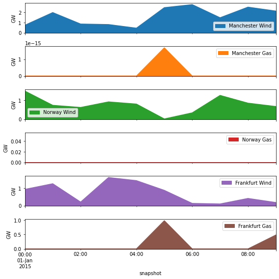
The wind generators have a per unit limit for each time step, given by the weather potentials at the site.
[9]:
network.generators_t.p_max_pu.plot.area(subplots=True)
plt.tight_layout()

Alright now we know how the network looks like, where the generators and lines are. Now, let’s perform a optimization of the operation and capacities.
[10]:
network.lopf();
INFO:pypsa.opf:Performed preliminary steps
INFO:pypsa.opf:Building pyomo model using `kirchhoff` formulation
INFO:pypsa.opf:Solving model using glpk
INFO:pypsa.opf:Optimization successful
# ==========================================================
# = Solver Results                                         =
# ==========================================================
# ----------------------------------------------------------
#   Problem Information
# ----------------------------------------------------------
Problem:
- Name: unknown
  Lower bound: -3474094.13081624
  Upper bound: -3474094.13081624
  Number of objectives: 1
  Number of constraints: 452
  Number of variables: 187
  Number of nonzeros: 971
  Sense: minimize
# ----------------------------------------------------------
#   Solver Information
# ----------------------------------------------------------
Solver:
- Status: ok
  Termination condition: optimal
  Statistics:
    Branch and bound:
      Number of bounded subproblems: 0
      Number of created subproblems: 0
  Error rc: 0
  Time: 0.011372089385986328
# ----------------------------------------------------------
#   Solution Information
# ----------------------------------------------------------
Solution:
- number of solutions: 0
  number of solutions displayed: 0
/home/docs/checkouts/readthedocs.org/user_builds/pypsa/conda/v0.19.3/lib/python3.10/site-packages/pypsa/opf.py:1971: FutureWarning: Using the level keyword in DataFrame and Series aggregations is deprecated and will be removed in a future version. Use groupby instead. df.sum(level=1) should use df.groupby(level=1).sum().
  pd.concat(
The objective is given by:
[11]:
network.objective
[11]:
-3474094.13081624
Why is this number negative? It considers the starting point of the optimization, thus the existent capacities given by network.generators.p_nom are taken into account.
The real system cost are given by
[12]:
network.objective + network.objective_constant
[12]:
18440973.387462903
The optimal capacities are given by p_nom_opt for generators, links and storages and s_nom_opt for lines.
Let’s look how the optimal capacities for the generators look like.
[13]:
network.generators.p_nom_opt.div(1e3).plot.bar(ylabel="GW", figsize=(8, 3))
plt.tight_layout()

Their production is again given as a time-series in network.generators_t.
[14]:
network.generators_t.p.div(1e3).plot.area(subplots=True, ylabel="GW")
plt.tight_layout()
What are the Locational Marginal Prices in the network. From the optimization these are given for each bus and snapshot.
[15]:
network.buses_t.marginal_price.mean(1).plot.area(figsize=(8, 3), ylabel="Euro per MWh")
plt.tight_layout()

We can inspect futher quantities as the active power of AC-DC converters and HVDC link.
[16]:
network.links_t.p0
[16]:
| Link | Norwich Converter | Norway Converter | Bremen Converter | DC link |
|---|---|---|---|---|
| snapshot | ||||
| 2015-01-01 00:00:00 | -316.117092 | 674.584826 | -358.467734 | -252.722217 |
| 2015-01-01 01:00:00 | 93.671942 | -116.727192 | 23.055250 | -96.601322 |
| 2015-01-01 02:00:00 | -285.234363 | 581.970687 | -296.736325 | 317.997991 |
| 2015-01-01 03:00:00 | -127.723339 | 272.557949 | -144.834610 | -276.046800 |
| 2015-01-01 04:00:00 | 37.371395 | -79.749487 | 42.378092 | -38.002664 |
| 2015-01-01 05:00:00 | 231.585916 | -494.197717 | 262.611801 | -162.836280 |
| 2015-01-01 06:00:00 | 900.000000 | -257.520720 | -642.479280 | 317.997991 |
| 2015-01-01 07:00:00 | 123.677319 | 971.918845 | -1095.596165 | -86.858742 |
| 2015-01-01 08:00:00 | 244.715828 | 850.880337 | -1095.596165 | 317.997991 |
| 2015-01-01 09:00:00 | 441.610034 | -86.851803 | -354.758231 | 294.728014 |
[17]:
network.lines_t.p0
[17]:
| Line | 0 | 1 | 2 | 3 | 4 | 5 | 6 |
|---|---|---|---|---|---|---|---|
| snapshot | |||||||
| 2015-01-01 00:00:00 | 68.553227 | -49.027273 | 0.000000 | -316.117092 | 358.467734 | -148.372745 | -534.340860 |
| 2015-01-01 01:00:00 | -486.507301 | 749.994027 | -31.623657 | 62.048285 | -54.678907 | 393.715939 | -823.210906 |
| 2015-01-01 02:00:00 | -287.678472 | 414.148821 | 10.156889 | -275.077474 | 306.893213 | 280.906831 | 173.898185 |
| 2015-01-01 03:00:00 | -52.491649 | 227.450897 | 0.000000 | -127.723339 | 144.834610 | -197.785304 | -743.788495 |
| 2015-01-01 04:00:00 | -120.055592 | 248.573165 | 0.000000 | 37.371395 | -42.378092 | -6.958088 | -883.817538 |
| 2015-01-01 05:00:00 | -620.461143 | 1172.121810 | 0.000000 | 231.585916 | -262.611801 | 148.559628 | -1030.848768 |
| 2015-01-01 06:00:00 | -661.294714 | 1378.422245 | -632.371427 | 267.628573 | 10.107853 | -53.448436 | 319.386680 |
| 2015-01-01 07:00:00 | -383.768641 | 540.906725 | -469.925715 | -346.248396 | 625.670450 | 393.715939 | 600.728881 |
| 2015-01-01 08:00:00 | -778.280943 | 1444.069207 | -522.116240 | -277.400413 | 573.479924 | 229.294311 | 501.346379 |
| 2015-01-01 09:00:00 | -528.891061 | 836.250807 | -325.313399 | 116.296635 | 29.444832 | 393.715939 | -248.566847 |
…or the active power injection per bus.
[18]:
network.buses_t.p
[18]:
| Bus | London | Norwich | Norwich DC | Manchester | Bremen | Bremen DC | Frankfurt | Norway | Norway DC |
|---|---|---|---|---|---|---|---|---|---|
| snapshot | |||||||||
| 2015-01-01 00:00:00 | 216.925973 | -99.345473 | -316.117092 | -117.580500 | -534.340860 | -358.467734 | 534.340860 | 3.979039e-12 | 674.584826 |
| 2015-01-01 01:00:00 | -880.223240 | -356.278088 | 93.671942 | 1236.501328 | -823.210906 | 23.055250 | 823.210906 | 4.263256e-14 | -116.727192 |
| 2015-01-01 02:00:00 | -568.585303 | -133.241990 | -285.234363 | 701.827293 | 173.898185 | -296.736325 | -173.898185 | -1.136868e-13 | 581.970687 |
| 2015-01-01 03:00:00 | 145.293655 | -425.236201 | -127.723339 | 279.942546 | -743.788495 | -144.834610 | 743.788495 | 0.000000e+00 | 272.557949 |
| 2015-01-01 04:00:00 | -113.097504 | -255.531253 | 37.371395 | 368.628757 | -883.817538 | 42.378092 | 883.817538 | -1.421085e-14 | -79.749487 |
| 2015-01-01 05:00:00 | -769.020772 | -1023.562182 | 231.585916 | 1792.582954 | -1030.848768 | 262.611801 | 1030.848768 | -5.684342e-14 | -494.197717 |
| 2015-01-01 06:00:00 | -607.846278 | -1431.870681 | 900.000000 | 2039.716959 | 319.386680 | -642.479280 | -319.386680 | -5.684342e-14 | -257.520720 |
| 2015-01-01 07:00:00 | -777.484580 | -147.190786 | 123.677319 | 924.675366 | 600.728881 | -1095.596165 | -600.728881 | 5.002221e-12 | 971.918845 |
| 2015-01-01 08:00:00 | -1007.575254 | -1214.774896 | 244.715828 | 2222.350150 | 501.346379 | -1095.596165 | -501.346379 | 0.000000e+00 | 850.880337 |
| 2015-01-01 09:00:00 | -922.607000 | -442.534868 | 441.610034 | 1365.141868 | -248.566847 | -354.758231 | 248.566847 | -2.273737e-13 | -86.851803 |