Two chained reservoirs

Two disconnected electrical loads are fed from two reservoirs linked by a river; the first reservoir has inflow from rain onto a water basin.

Note that the two reservoirs are tightly coupled, meaning there is no time delay between the first one emptying and the second one filling, as there would be if there were a long stretch of river between the reservoirs. The reservoirs are essentially assumed to be close to each other. A time delay would require a “Link” element between different snapshots, which is not yet supported by PyPSA (but could be enabled by passing network.lopf() an extra_functionality function).

[1]:

import pypsa
import pandas as pd
import numpy as np
import matplotlib.pyplot as plt

from pyomo.environ import Constraint

First tell PyPSA that links will have a 2nd bus by overriding the component_attrs. This is needed so that water can both go through a turbine AND feed the next reservoir

[2]:

override_component_attrs = pypsa.descriptors.Dict(
    {k: v.copy() for k, v in pypsa.components.component_attrs.items()}
)
override_component_attrs["Link"].loc["bus2"] = [
    "string",
    np.nan,
    np.nan,
    "2nd bus",
    "Input (optional)",
]
override_component_attrs["Link"].loc["efficiency2"] = [
    "static or series",
    "per unit",
    1.0,
    "2nd bus efficiency",
    "Input (optional)",
]
override_component_attrs["Link"].loc["p2"] = [
    "series",
    "MW",
    0.0,
    "2nd bus output",
    "Output",
]

[3]:

network = pypsa.Network(override_component_attrs=override_component_attrs)
network.set_snapshots(pd.date_range("2016-01-01 00:00", "2016-01-01 03:00", freq="H"))

Add assets to the network.

[4]:

network.add("Carrier", "reservoir")
network.add("Carrier", "rain")

network.add("Bus", "0", carrier="AC")
network.add("Bus", "1", carrier="AC")

network.add("Bus", "0 reservoir", carrier="reservoir")
network.add("Bus", "1 reservoir", carrier="reservoir")


network.add(
    "Generator",
    "rain",
    bus="0 reservoir",
    carrier="rain",
    p_nom=1000,
    p_max_pu=[0.0, 0.2, 0.7, 0.4],
)


network.add("Load", "0 load", bus="0", p_set=20.0)

network.add("Load", "1 load", bus="1", p_set=30.0)

The efficiency of a river is the relation between the gravitational potential energy of 1 m^3 of water in reservoir 0 relative to its turbine versus the potential energy of 1 m^3 of water in reservoir 1 relative to its turbine

[5]:

network.add(
    "Link",
    "spillage",
    bus0="0 reservoir",
    bus1="1 reservoir",
    efficiency=0.5,
    p_nom_extendable=True,
)


# water from turbine also goes into next reservoir
network.add(
    "Link",
    "0 turbine",
    bus0="0 reservoir",
    bus1="0",
    bus2="1 reservoir",
    efficiency=0.9,
    efficiency2=0.5,
    capital_cost=1000,
    p_nom_extendable=True,
)

network.add(
    "Link",
    "1 turbine",
    bus0="1 reservoir",
    bus1="1",
    efficiency=0.9,
    capital_cost=1000,
    p_nom_extendable=True,
)


network.add(
    "Store", "0 reservoir", bus="0 reservoir", e_cyclic=True, e_nom_extendable=True
)

network.add(
    "Store", "1 reservoir", bus="1 reservoir", e_cyclic=True, e_nom_extendable=True
)

[6]:

network.lopf(network.snapshots)
print("Objective:", network.objective)

WARNING:pypsa.components:Solving optimisation problem with pyomo.In PyPSA version 0.21 the default will change to ``n.lopf(pyomo=False)``.Explicitly set ``n.lopf(pyomo=True)`` to retain current behaviour.
INFO:pypsa.opf:Performed preliminary steps
INFO:pypsa.opf:Building pyomo model using `kirchhoff` formulation
INFO:pypsa.opf:Solving model using glpk
INFO:pypsa.opf:Optimization successful

# ==========================================================
# = Solver Results                                         =
# ==========================================================
# ----------------------------------------------------------
#   Problem Information
# ----------------------------------------------------------
Problem:
- Name: unknown
  Lower bound: 55555.5555555556
  Upper bound: 55555.5555555556
  Number of objectives: 1
  Number of constraints: 65
  Number of variables: 38
  Number of nonzeros: 125
  Sense: minimize
# ----------------------------------------------------------
#   Solver Information
# ----------------------------------------------------------
Solver:
- Status: ok
  Termination condition: optimal
  Statistics:
    Branch and bound:
      Number of bounded subproblems: 0
      Number of created subproblems: 0
  Error rc: 0
  Time: 0.002696514129638672
# ----------------------------------------------------------
#   Solution Information
# ----------------------------------------------------------
Solution:
- number of solutions: 0
  number of solutions displayed: 0
Objective: 55555.5555555556

[7]:

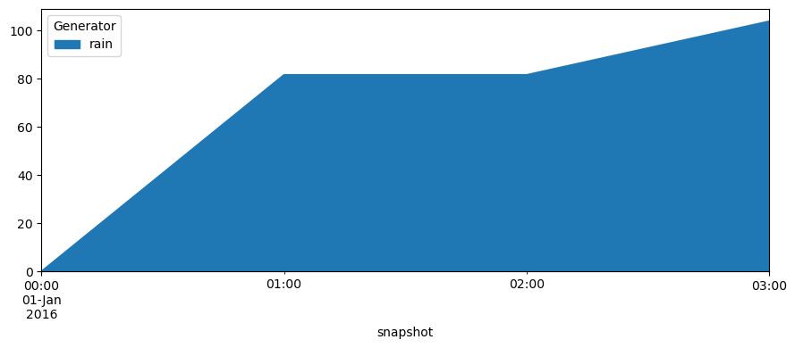
network.generators_t.p.plot.area(figsize=(9, 4))
plt.tight_layout()

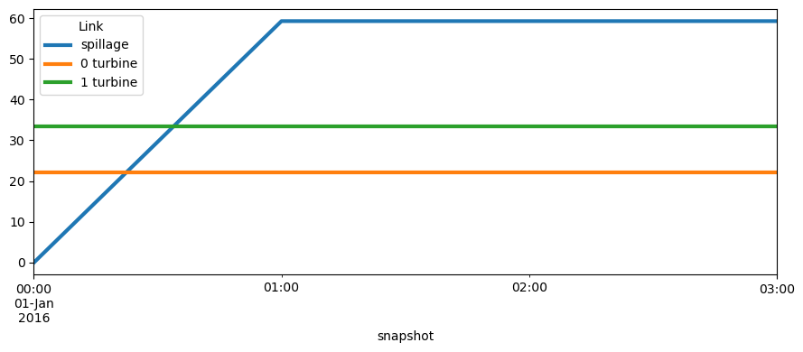
../_images/examples_chained-hydro-reservoirs_10_0.png

Now, let’s have look at the different outputs of the links.

[8]:

network.links_t.p0.plot(figsize=(9, 4), lw=3)
plt.tight_layout()

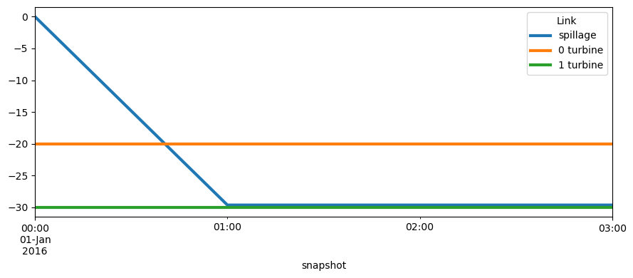
../_images/examples_chained-hydro-reservoirs_12_0.png

[9]:

network.links_t.p1.plot(figsize=(9, 4), lw=3)
plt.tight_layout()

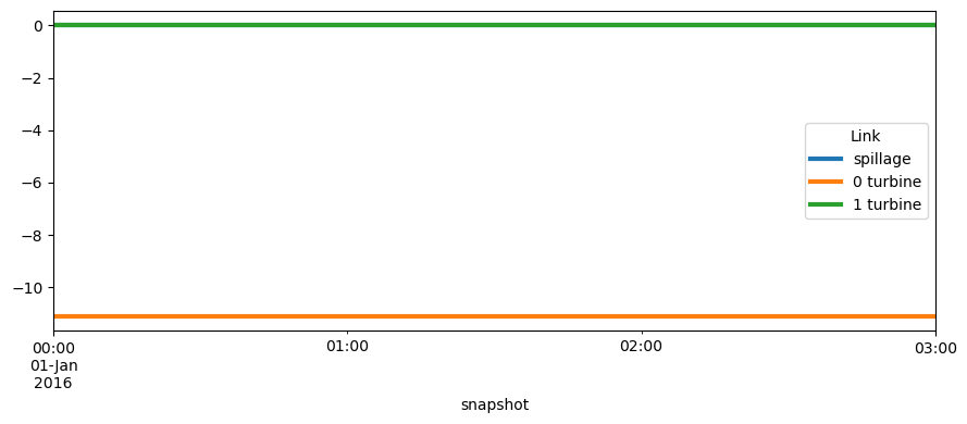
../_images/examples_chained-hydro-reservoirs_13_0.png

[10]:

network.links_t.p2.plot(figsize=(9, 4), lw=3)
plt.tight_layout()

../_images/examples_chained-hydro-reservoirs_14_0.png

What are the energy outputs and energy levels at the reservoirs?

[11]:

pd.DataFrame({attr: network.stores_t[attr]["0 reservoir"] for attr in ["p", "e"]})

[11]:

	p	e
snapshot
2016-01-01 00:00:00	22.222222	0.000000
2016-01-01 01:00:00	0.000000	0.000000
2016-01-01 02:00:00	0.000000	0.000000
2016-01-01 03:00:00	-22.222222	22.222222

[12]:

pd.DataFrame({attr: network.stores_t[attr]["1 reservoir"] for attr in ["p", "e"]})

[12]:

	p	e
snapshot
2016-01-01 00:00:00	22.222222	0.000000
2016-01-01 01:00:00	-7.407407	7.407407
2016-01-01 02:00:00	-7.407407	14.814815
2016-01-01 03:00:00	-7.407407	22.222222