Note
You can download this example as a Jupyter notebook or start it in interactive mode.
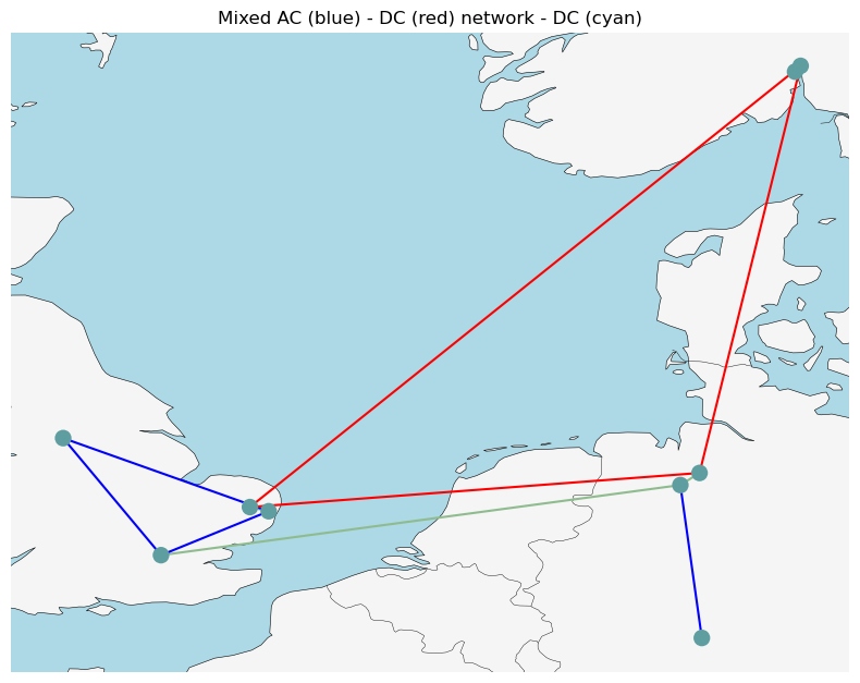
Meshed AC-DC example
This example has a 3-node AC network coupled via AC-DC converters to a 3-node DC network. There is also a single point-to-point DC using the Link component.
The data files for this example are in the examples folder of the github repository: https://github.com/PyPSA/PyPSA.
[1]:
import pypsa
import numpy as np
import pandas as pd
import os
import matplotlib.pyplot as plt
import cartopy.crs as ccrs

%matplotlib inline
plt.rc("figure", figsize=(8, 8))
[2]:
network = pypsa.examples.ac_dc_meshed(from_master=True)
WARNING:pypsa.io:Importing network from PyPSA version v0.17.1 while current version is v0.21.1. Read the release notes at https://pypsa.readthedocs.io/en/latest/release_notes.html to prepare your network for import.
INFO:pypsa.io:Imported network ac-dc-meshed.nc has buses, carriers, generators, global_constraints, lines, links, loads
[3]:
# get current type (AC or DC) of the lines from the buses
lines_current_type = network.lines.bus0.map(network.buses.carrier)
lines_current_type
[3]:
Line
0    AC
1    AC
2    DC
3    DC
4    DC
5    AC
6    AC
Name: bus0, dtype: object
[4]:
network.plot(
    line_colors=lines_current_type.map(lambda ct: "r" if ct == "DC" else "b"),
    title="Mixed AC (blue) - DC (red) network - DC (cyan)",
    color_geomap=True,
    jitter=0.3,
)
plt.tight_layout()
/home/docs/checkouts/readthedocs.org/user_builds/pypsa/conda/v0.21.1/lib/python3.10/site-packages/cartopy/io/__init__.py:241: DownloadWarning: Downloading: https://naturalearth.s3.amazonaws.com/50m_physical/ne_50m_land.zip
  warnings.warn(f'Downloading: {url}', DownloadWarning)
/home/docs/checkouts/readthedocs.org/user_builds/pypsa/conda/v0.21.1/lib/python3.10/site-packages/cartopy/io/__init__.py:241: DownloadWarning: Downloading: https://naturalearth.s3.amazonaws.com/50m_physical/ne_50m_ocean.zip
  warnings.warn(f'Downloading: {url}', DownloadWarning)
/home/docs/checkouts/readthedocs.org/user_builds/pypsa/conda/v0.21.1/lib/python3.10/site-packages/cartopy/io/__init__.py:241: DownloadWarning: Downloading: https://naturalearth.s3.amazonaws.com/50m_cultural/ne_50m_admin_0_boundary_lines_land.zip
  warnings.warn(f'Downloading: {url}', DownloadWarning)
/home/docs/checkouts/readthedocs.org/user_builds/pypsa/conda/v0.21.1/lib/python3.10/site-packages/cartopy/io/__init__.py:241: DownloadWarning: Downloading: https://naturalearth.s3.amazonaws.com/50m_physical/ne_50m_coastline.zip
  warnings.warn(f'Downloading: {url}', DownloadWarning)
[5]:
network.links.loc["Norwich Converter", "p_nom_extendable"] = False
We inspect the topology of the network. Therefore use the function determine_network_topology and inspect the subnetworks in network.sub_networks.
[6]:
network.determine_network_topology()
network.sub_networks["n_branches"] = [
    len(sn.branches()) for sn in network.sub_networks.obj
]
network.sub_networks["n_buses"] = [len(sn.buses()) for sn in network.sub_networks.obj]

network.sub_networks
[6]:
| attribute | carrier | slack_bus | obj | n_branches | n_buses |
|---|---|---|---|---|---|
| SubNetwork | |||||
| 0 | AC | Manchester | SubNetwork 0 | 3 | 3 |
| 1 | DC | Norwich DC | SubNetwork 1 | 3 | 3 |
| 2 | AC | Frankfurt | SubNetwork 2 | 1 | 2 |
| 3 | AC | Norway | SubNetwork 3 | 0 | 1 |
The network covers 10 time steps. These are given by the snapshots attribute.
[7]:
network.snapshots
[7]:
DatetimeIndex(['2015-01-01 00:00:00', '2015-01-01 01:00:00',
               '2015-01-01 02:00:00', '2015-01-01 03:00:00',
               '2015-01-01 04:00:00', '2015-01-01 05:00:00',
               '2015-01-01 06:00:00', '2015-01-01 07:00:00',
               '2015-01-01 08:00:00', '2015-01-01 09:00:00'],
              dtype='datetime64[ns]', name='snapshot', freq=None)
There are 6 generators in the network, 3 wind and 3 gas. All are attached to buses:
[8]:
network.generators
[8]:
| bus | capital_cost | efficiency | marginal_cost | p_nom | p_nom_extendable | p_nom_min | carrier | control | type | ... | shut_down_cost | min_up_time | min_down_time | up_time_before | down_time_before | ramp_limit_up | ramp_limit_down | ramp_limit_start_up | ramp_limit_shut_down | p_nom_opt | |
|---|---|---|---|---|---|---|---|---|---|---|---|---|---|---|---|---|---|---|---|---|---|
| Generator | |||||||||||||||||||||
| Manchester Wind | Manchester | 2793.651603 | 1.000000 | 0.110000 | 80.0 | True | 100.0 | wind | Slack | ... | 0.0 | 0 | 0 | 1 | 0 | NaN | NaN | 1.0 | 1.0 | 0.0 | |
| Manchester Gas | Manchester | 196.615168 | 0.350026 | 4.532368 | 50000.0 | True | 0.0 | gas | PQ | ... | 0.0 | 0 | 0 | 1 | 0 | NaN | NaN | 1.0 | 1.0 | 0.0 | |
| Norway Wind | Norway | 2184.374796 | 1.000000 | 0.090000 | 100.0 | True | 100.0 | wind | Slack | ... | 0.0 | 0 | 0 | 1 | 0 | NaN | NaN | 1.0 | 1.0 | 0.0 | |
| Norway Gas | Norway | 158.251250 | 0.356836 | 5.892845 | 20000.0 | True | 0.0 | gas | PQ | ... | 0.0 | 0 | 0 | 1 | 0 | NaN | NaN | 1.0 | 1.0 | 0.0 | |
| Frankfurt Wind | Frankfurt | 2129.456122 | 1.000000 | 0.100000 | 110.0 | True | 100.0 | wind | Slack | ... | 0.0 | 0 | 0 | 1 | 0 | NaN | NaN | 1.0 | 1.0 | 0.0 | |
| Frankfurt Gas | Frankfurt | 102.676953 | 0.351666 | 4.086322 | 80000.0 | True | 0.0 | gas | PQ | ... | 0.0 | 0 | 0 | 1 | 0 | NaN | NaN | 1.0 | 1.0 | 0.0 |
6 rows × 30 columns
We see that the generators have different capital and marginal costs. All of them have a p_nom_extendable set to True, meaning that capacities can be extended in the optimization.
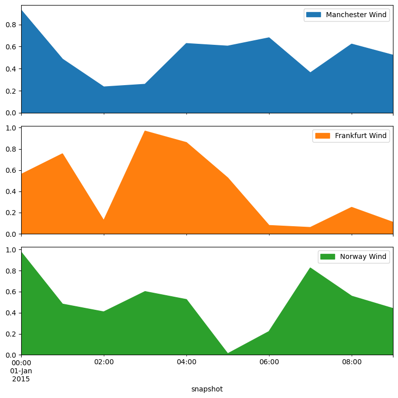
The wind generators have a per unit limit for each time step, given by the weather potentials at the site.
[9]:
network.generators_t.p_max_pu.plot.area(subplots=True)
plt.tight_layout()
Alright now we know how the network looks like, where the generators and lines are. Now, let’s perform a optimization of the operation and capacities.
[10]:
network.lopf(pyomo=False);
INFO:pypsa.linopf:Prepare linear problem
/home/docs/checkouts/readthedocs.org/user_builds/pypsa/conda/v0.21.1/lib/python3.10/site-packages/pypsa/linopt.py:474: FutureWarning: In a future version, `df.iloc[:, i] = newvals` will attempt to set the values inplace instead of always setting a new array. To retain the old behavior, use either `df[df.columns[i]] = newvals` or, if columns are non-unique, `df.isetitem(i, newvals)`
  ref_dict.pnl[attr].loc[df.index, df.columns] = df
INFO:pypsa.linopf:Total preparation time: 0.21s
INFO:pypsa.linopf:Solve linear problem using Glpk solver
INFO:pypsa.linopf:Optimization successful. Objective value: -3.47e+06
The objective is given by:
[11]:
network.objective
[11]:
-3474092.381
Why is this number negative? It considers the starting point of the optimization, thus the existent capacities given by network.generators.p_nom are taken into account.
The real system cost are given by
[12]:
network.objective + network.objective_constant
[12]:
18440975.13727914
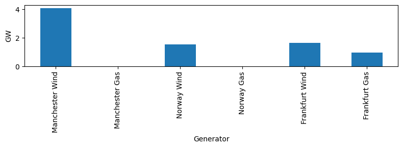
The optimal capacities are given by p_nom_opt for generators, links and storages and s_nom_opt for lines.
Let’s look how the optimal capacities for the generators look like.
[13]:
network.generators.p_nom_opt.div(1e3).plot.bar(ylabel="GW", figsize=(8, 3))
plt.tight_layout()
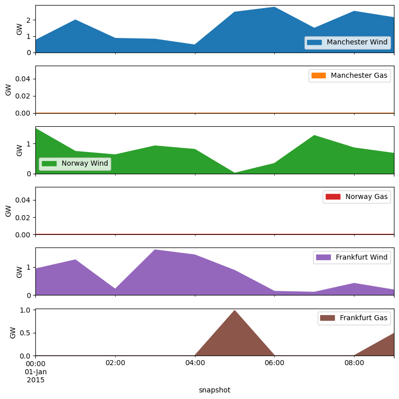
Their production is again given as a time-series in network.generators_t.
[14]:
network.generators_t.p.div(1e3).plot.area(subplots=True, ylabel="GW")
plt.tight_layout()
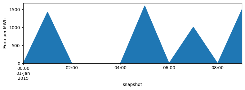
What are the Locational Marginal Prices in the network. From the optimization these are given for each bus and snapshot.
[15]:
network.buses_t.marginal_price.mean(1).plot.area(figsize=(8, 3), ylabel="Euro per MWh")
plt.tight_layout()
We can inspect futher quantities as the active power of AC-DC converters and HVDC link.
[16]:
network.links_t.p0
[16]:
| Link | Norwich Converter | Norway Converter | Bremen Converter | DC link |
|---|---|---|---|---|
| snapshot | ||||
| 2015-01-01 00:00:00 | -250.8340 | 674.5810 | -423.746 | -317.9990 |
| 2015-01-01 01:00:00 | 315.0740 | -116.7300 | -198.344 | -317.9990 |
| 2015-01-01 02:00:00 | -285.2340 | 581.9690 | -296.735 | 317.9990 |
| 2015-01-01 03:00:00 | -85.7678 | 272.5560 | -186.788 | -317.9990 |
| 2015-01-01 04:00:00 | 317.3710 | -79.7518 | -237.619 | -317.9990 |
| 2015-01-01 05:00:00 | 386.7500 | -494.1970 | 107.447 | -317.9990 |
| 2015-01-01 06:00:00 | 900.0000 | -257.5220 | -642.478 | 317.9990 |
| 2015-01-01 07:00:00 | 123.6790 | 971.9160 | -1095.600 | -86.8575 |
| 2015-01-01 08:00:00 | 244.7170 | 850.8790 | -1095.600 | 317.9990 |
| 2015-01-01 09:00:00 | 820.0230 | -86.8535 | -733.169 | -83.6841 |
[17]:
network.lines_t.p0
[17]:
| Line | 0 | 1 | 2 | 3 | 4 | 5 | 6 |
|---|---|---|---|---|---|---|---|
| snapshot | |||||||
| 2015-01-01 00:00:00 | 79.4736 | -38.1015 | -52.9713 | -303.806 | 370.7750 | -202.7300 | -534.340 |
| 2015-01-01 01:00:00 | -449.4640 | 787.0410 | -211.2770 | 103.798 | -12.9321 | 209.3610 | -823.209 |
| 2015-01-01 02:00:00 | -287.6790 | 414.1500 | 10.1573 | -275.077 | 306.8920 | 280.9080 | 173.898 |
| 2015-01-01 03:00:00 | -45.4730 | 234.4720 | -34.0434 | -119.811 | 152.7440 | -232.7190 | -743.788 |
| 2015-01-01 04:00:00 | -73.2083 | 295.4240 | -227.2010 | 90.170 | 10.4182 | -240.1080 | -883.817 |
| 2015-01-01 05:00:00 | -594.4990 | 1198.0800 | -125.9060 | 260.844 | -233.3530 | 19.3581 | -1030.850 |
| 2015-01-01 06:00:00 | -661.2950 | 1378.4200 | -632.3710 | 267.629 | 10.1069 | -53.4469 | 319.387 |
| 2015-01-01 07:00:00 | -383.7690 | 540.9090 | -469.9270 | -346.247 | 625.6690 | 393.7160 | 600.730 |
| 2015-01-01 08:00:00 | -778.2810 | 1444.0700 | -522.1170 | -277.400 | 573.4790 | 229.2960 | 501.348 |
| 2015-01-01 09:00:00 | -465.5760 | 899.5660 | -632.3710 | 187.652 | 100.7980 | 78.6186 | -248.568 |
…or the active power injection per bus.
[18]:
network.buses_t.p
[18]:
| Bus | London | Norwich | Norwich DC | Manchester | Bremen | Bremen DC | Frankfurt | Norway | Norway DC |
|---|---|---|---|---|---|---|---|---|---|
| snapshot | |||||||||
| 2015-01-01 00:00:00 | 282.202756 | -164.628564 | -250.8340 | -117.575440 | -534.339378 | -423.746 | 534.339153 | 0.003164 | 674.5810 |
| 2015-01-01 01:00:00 | -658.825561 | -577.680146 | 315.0740 | 1236.500376 | -823.209334 | -198.344 | 823.213894 | -0.000047 | -116.7300 |
| 2015-01-01 02:00:00 | -568.586312 | -133.242353 | -285.2340 | 701.829124 | 173.897870 | -296.735 | -173.898928 | 0.000256 | 581.9690 |
| 2015-01-01 03:00:00 | 187.245855 | -467.191739 | -85.7678 | 279.945178 | -743.787306 | -186.788 | 743.788236 | -0.000233 | 272.5560 |
| 2015-01-01 04:00:00 | 166.898831 | -535.530858 | 317.3710 | 368.632241 | -883.816781 | -237.619 | 883.819245 | -0.000073 | -79.7518 |
| 2015-01-01 05:00:00 | -613.858052 | -1178.726266 | 386.7500 | 1792.586681 | -1030.846687 | 107.447 | 1030.846757 | -0.000349 | -494.1970 |
| 2015-01-01 06:00:00 | -607.847287 | -1431.870681 | 900.0000 | 2039.722900 | 319.386410 | -642.478 | -319.386752 | 0.000035 | -257.5220 |
| 2015-01-01 07:00:00 | -777.485822 | -147.192467 | 123.6790 | 924.675111 | 600.733959 | -1095.600 | -600.729766 | 0.001550 | 971.9160 |
| 2015-01-01 08:00:00 | -1007.576264 | -1214.776068 | 244.7170 | 2222.351918 | 501.351224 | -1095.600 | -501.347780 | -0.000493 | 850.8790 |
| 2015-01-01 09:00:00 | -544.194886 | -820.947834 | 820.0230 | 1365.139414 | -248.568192 | -733.169 | 248.567354 | 0.000323 | -86.8535 |