Note
You can download this example as a Jupyter notebook or start it in interactive mode.
Meshed AC-DC example#
This example has a 3-node AC network coupled via AC-DC converters to a 3-node DC network. There is also a single point-to-point DC using the Link component.
The data files for this example are in the examples folder of the github repository: PyPSA/PyPSA.
[1]:
import pypsa
import numpy as np
import pandas as pd
import os
import matplotlib.pyplot as plt
import cartopy.crs as ccrs

%matplotlib inline
plt.rc("figure", figsize=(8, 8))
ERROR 1: PROJ: proj_create_from_database: Open of /home/docs/checkouts/readthedocs.org/user_builds/pypsa/conda/latest/share/proj failed
[2]:
network = pypsa.examples.ac_dc_meshed(from_master=True)
WARNING:pypsa.io:Importing network from PyPSA version v0.17.1 while current version is v0.28.0. Read the release notes at https://pypsa.readthedocs.io/en/latest/release_notes.html to prepare your network for import.
INFO:pypsa.io:Imported network ac-dc-meshed.nc has buses, carriers, generators, global_constraints, lines, links, loads
[3]:
# get current type (AC or DC) of the lines from the buses
lines_current_type = network.lines.bus0.map(network.buses.carrier)
lines_current_type
[3]:
Line
0    AC
1    AC
2    DC
3    DC
4    DC
5    AC
6    AC
Name: bus0, dtype: object
[4]:
network.plot(
    line_colors=lines_current_type.map(lambda ct: "r" if ct == "DC" else "b"),
    title="Mixed AC (blue) - DC (red) network - DC (cyan)",
    color_geomap=True,
    jitter=0.3,
)
plt.tight_layout()
/home/docs/checkouts/readthedocs.org/user_builds/pypsa/conda/latest/lib/python3.11/site-packages/cartopy/mpl/feature_artist.py:144: UserWarning: facecolor will have no effect as it has been defined as "never".
  warnings.warn('facecolor will have no effect as it has been '
/home/docs/checkouts/readthedocs.org/user_builds/pypsa/conda/latest/lib/python3.11/site-packages/cartopy/io/__init__.py:241: DownloadWarning: Downloading: https://naturalearth.s3.amazonaws.com/50m_physical/ne_50m_land.zip
  warnings.warn(f'Downloading: {url}', DownloadWarning)
/home/docs/checkouts/readthedocs.org/user_builds/pypsa/conda/latest/lib/python3.11/site-packages/cartopy/io/__init__.py:241: DownloadWarning: Downloading: https://naturalearth.s3.amazonaws.com/50m_physical/ne_50m_ocean.zip
  warnings.warn(f'Downloading: {url}', DownloadWarning)
/home/docs/checkouts/readthedocs.org/user_builds/pypsa/conda/latest/lib/python3.11/site-packages/cartopy/io/__init__.py:241: DownloadWarning: Downloading: https://naturalearth.s3.amazonaws.com/50m_cultural/ne_50m_admin_0_boundary_lines_land.zip
  warnings.warn(f'Downloading: {url}', DownloadWarning)
/home/docs/checkouts/readthedocs.org/user_builds/pypsa/conda/latest/lib/python3.11/site-packages/cartopy/io/__init__.py:241: DownloadWarning: Downloading: https://naturalearth.s3.amazonaws.com/50m_physical/ne_50m_coastline.zip
  warnings.warn(f'Downloading: {url}', DownloadWarning)

[5]:
network.links.loc["Norwich Converter", "p_nom_extendable"] = False
We inspect the topology of the network. Therefore use the function determine_network_topology and inspect the subnetworks in network.sub_networks.
[6]:
network.determine_network_topology()
network.sub_networks["n_branches"] = [
    len(sn.branches()) for sn in network.sub_networks.obj
]
network.sub_networks["n_buses"] = [len(sn.buses()) for sn in network.sub_networks.obj]

network.sub_networks
[6]:
| attribute | carrier | slack_bus | obj | n_branches | n_buses |
|---|---|---|---|---|---|
| SubNetwork | |||||
| 0 | AC | Manchester | SubNetwork 0 | 3 | 3 |
| 1 | DC | Norwich DC | SubNetwork 1 | 3 | 3 |
| 2 | AC | Frankfurt | SubNetwork 2 | 1 | 2 |
| 3 | AC | Norway | SubNetwork 3 | 0 | 1 |
The network covers 10 time steps. These are given by the snapshots attribute.
[7]:
network.snapshots
[7]:
DatetimeIndex(['2015-01-01 00:00:00', '2015-01-01 01:00:00',
               '2015-01-01 02:00:00', '2015-01-01 03:00:00',
               '2015-01-01 04:00:00', '2015-01-01 05:00:00',
               '2015-01-01 06:00:00', '2015-01-01 07:00:00',
               '2015-01-01 08:00:00', '2015-01-01 09:00:00'],
              dtype='datetime64[ns]', name='snapshot', freq=None)
There are 6 generators in the network, 3 wind and 3 gas. All are attached to buses:
[8]:
network.generators
[8]:
| bus | capital_cost | efficiency | marginal_cost | p_nom | p_nom_extendable | p_nom_min | carrier | control | type | ... | min_up_time | min_down_time | up_time_before | down_time_before | ramp_limit_up | ramp_limit_down | ramp_limit_start_up | ramp_limit_shut_down | weight | p_nom_opt | |
|---|---|---|---|---|---|---|---|---|---|---|---|---|---|---|---|---|---|---|---|---|---|
| Generator | |||||||||||||||||||||
| Manchester Wind | Manchester | 2793.651603 | 1.000000 | 0.110000 | 80.0 | True | 100.0 | wind | Slack | ... | 0 | 0 | 1 | 0 | NaN | NaN | 1.0 | 1.0 | 1.0 | 0.0 | |
| Manchester Gas | Manchester | 196.615168 | 0.350026 | 4.532368 | 50000.0 | True | 0.0 | gas | PQ | ... | 0 | 0 | 1 | 0 | NaN | NaN | 1.0 | 1.0 | 1.0 | 0.0 | |
| Norway Wind | Norway | 2184.374796 | 1.000000 | 0.090000 | 100.0 | True | 100.0 | wind | Slack | ... | 0 | 0 | 1 | 0 | NaN | NaN | 1.0 | 1.0 | 1.0 | 0.0 | |
| Norway Gas | Norway | 158.251250 | 0.356836 | 5.892845 | 20000.0 | True | 0.0 | gas | PQ | ... | 0 | 0 | 1 | 0 | NaN | NaN | 1.0 | 1.0 | 1.0 | 0.0 | |
| Frankfurt Wind | Frankfurt | 2129.456122 | 1.000000 | 0.100000 | 110.0 | True | 100.0 | wind | Slack | ... | 0 | 0 | 1 | 0 | NaN | NaN | 1.0 | 1.0 | 1.0 | 0.0 | |
| Frankfurt Gas | Frankfurt | 102.676953 | 0.351666 | 4.086322 | 80000.0 | True | 0.0 | gas | PQ | ... | 0 | 0 | 1 | 0 | NaN | NaN | 1.0 | 1.0 | 1.0 | 0.0 |
6 rows × 34 columns
We see that the generators have different capital and marginal costs. All of them have a p_nom_extendable set to True, meaning that capacities can be extended in the optimization.
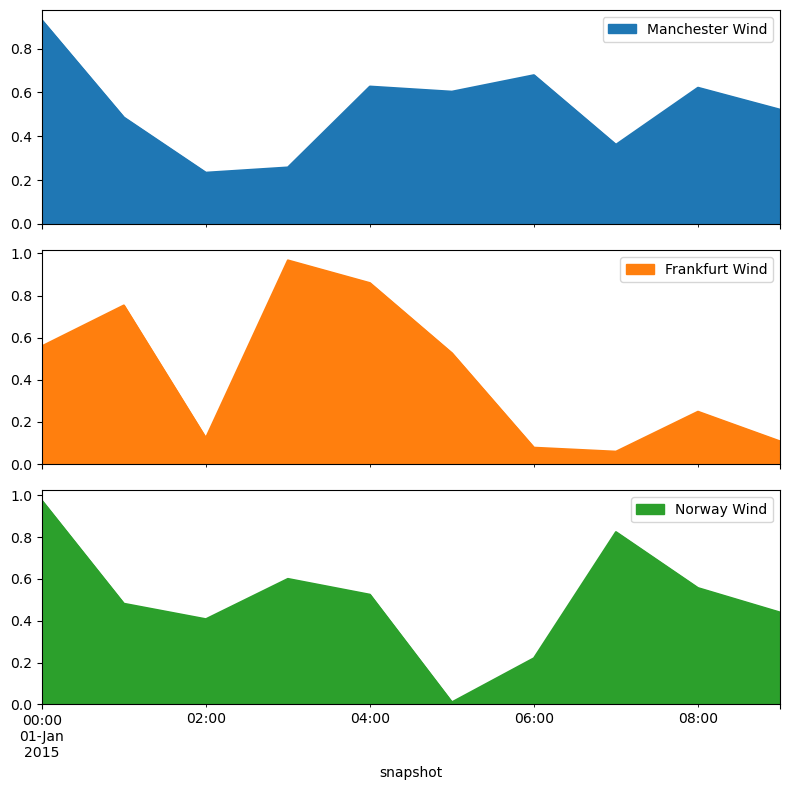
The wind generators have a per unit limit for each time step, given by the weather potentials at the site.
[9]:
network.generators_t.p_max_pu.plot.area(subplots=True)
plt.tight_layout()
Alright now we know how the network looks like, where the generators and lines are. Now, let’s perform a optimization of the operation and capacities.
[10]:
network.optimize();
WARNING:pypsa.components:The following lines have zero x, which could break the linear load flow:
Index(['2', '3', '4'], dtype='object', name='Line')
WARNING:pypsa.components:The following lines have zero r, which could break the linear load flow:
Index(['0', '1', '5', '6'], dtype='object', name='Line')
INFO:linopy.model: Solve problem using Glpk solver
INFO:linopy.io: Writing time: 0.07s
INFO:linopy.solvers:GLPSOL--GLPK LP/MIP Solver 5.0
Parameter(s) specified in the command line:
 --lp /tmp/linopy-problem-mblw2kbv.lp --output /tmp/linopy-solve-piw918bx.sol
Reading problem data from '/tmp/linopy-problem-mblw2kbv.lp'...
467 rows, 187 columns, 986 non-zeros
2650 lines were read
GLPK Simplex Optimizer 5.0
467 rows, 187 columns, 986 non-zeros
Preprocessing...
371 rows, 186 columns, 890 non-zeros
Scaling...
 A: min|aij| =  9.693e-03  max|aij| =  1.215e+00  ratio =  1.254e+02
GM: min|aij| =  5.786e-01  max|aij| =  1.728e+00  ratio =  2.987e+00
EQ: min|aij| =  3.378e-01  max|aij| =  1.000e+00  ratio =  2.961e+00
Constructing initial basis...
Size of triangular part is 371
      0: obj =  -2.104300118e+07 inf =   9.187e+04 (92)
    165: obj =   8.711702088e+06 inf =   1.017e-11 (0) 1
*   245: obj =  -3.474094131e+06 inf =   0.000e+00 (0) 1
OPTIMAL LP SOLUTION FOUND
Time used:   0.0 secs
Memory used: 0.6 Mb (632037 bytes)
Writing basic solution to '/tmp/linopy-solve-piw918bx.sol'...

INFO:linopy.constants: Optimization successful:
Status: ok
Termination condition: optimal
Solution: 187 primals, 467 duals
Objective: -3.47e+06
Solver model: not available
Solver message: optimal

INFO:pypsa.optimization.optimize:The shadow-prices of the constraints Generator-ext-p-lower, Generator-ext-p-upper, Line-ext-s-lower, Line-ext-s-upper, Link-fix-p-lower, Link-fix-p-upper, Link-ext-p-lower, Link-ext-p-upper, Kirchhoff-Voltage-Law were not assigned to the network.
The objective is given by:
[11]:
network.objective
[11]:
-3474094.131
Why is this number negative? It considers the starting point of the optimization, thus the existent capacities given by network.generators.p_nom are taken into account.
The real system cost are given by
[12]:
network.objective + network.objective_constant
[12]:
18440973.38727914
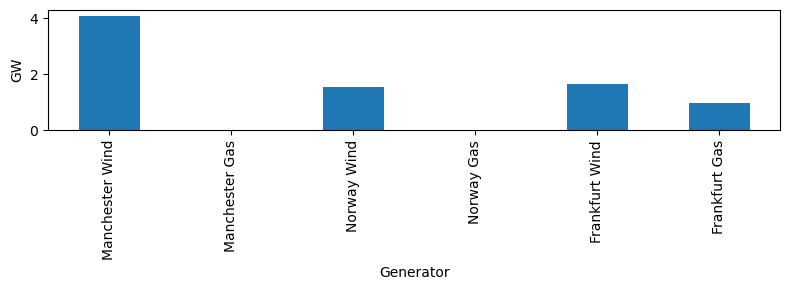
The optimal capacities are given by p_nom_opt for generators, links and storages and s_nom_opt for lines.
Let’s look how the optimal capacities for the generators look like.
[13]:
network.generators.p_nom_opt.div(1e3).plot.bar(ylabel="GW", figsize=(8, 3))
plt.tight_layout()
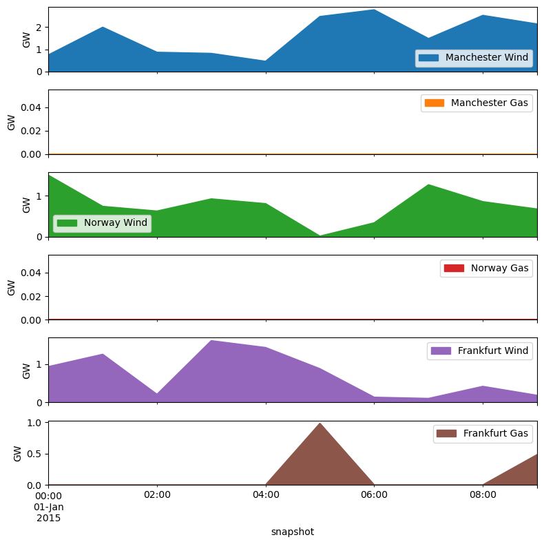
Their production is again given as a time-series in network.generators_t.
[14]:
network.generators_t.p.div(1e3).plot.area(subplots=True, ylabel="GW")
plt.tight_layout()
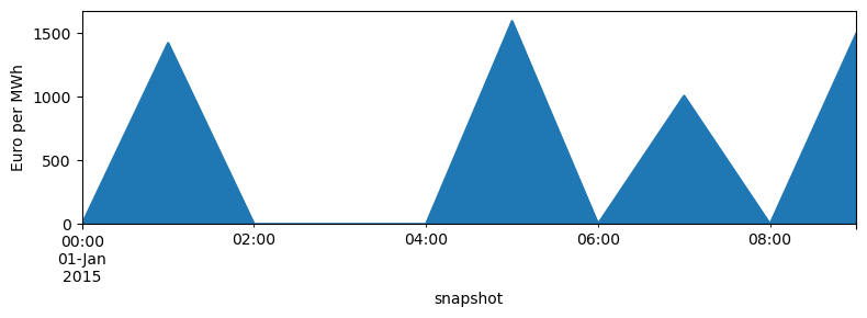
What are the Locational Marginal Prices in the network. From the optimization these are given for each bus and snapshot.
[15]:
network.buses_t.marginal_price.mean(1).plot.area(figsize=(8, 3), ylabel="Euro per MWh")
plt.tight_layout()
We can inspect further quantities as the active power of AC-DC converters and HVDC link.
[16]:
network.links_t.p0
[16]:
| Link | Norwich Converter | Norway Converter | Bremen Converter | DC link |
|---|---|---|---|---|
| snapshot | ||||
| 2015-01-01 00:00:00 | -250.8410 | 674.5850 | -423.7440 | -317.9980 |
| 2015-01-01 01:00:00 | 93.6719 | -116.7270 | 23.0553 | -96.6013 |
| 2015-01-01 02:00:00 | -285.2340 | 581.9710 | -296.7360 | 317.9980 |
| 2015-01-01 03:00:00 | -85.7721 | 272.5580 | -186.7860 | -317.9980 |
| 2015-01-01 04:00:00 | 317.3670 | -79.7495 | -237.6170 | -317.9980 |
| 2015-01-01 05:00:00 | 386.7480 | -494.1980 | 107.4500 | -317.9980 |
| 2015-01-01 06:00:00 | 900.0000 | -257.5210 | -642.4790 | 317.9980 |
| 2015-01-01 07:00:00 | 123.6770 | 971.9190 | -1095.6000 | -86.8587 |
| 2015-01-01 08:00:00 | 244.7160 | 850.8800 | -1095.6000 | 317.9980 |
| 2015-01-01 09:00:00 | 441.6100 | -86.8518 | -354.7580 | 294.7280 |
[17]:
network.lines_t.p0
[17]:
| Line | 0 | 1 | 2 | 3 | 4 | 5 | 6 |
|---|---|---|---|---|---|---|---|
| snapshot | |||||||
| 2015-01-01 00:00:00 | 79.4749 | -38.1056 | -52.9672 | -303.8080 | 370.7760 | -202.7270 | -534.341 |
| 2015-01-01 01:00:00 | -486.5070 | 749.9940 | -31.6237 | 62.0483 | -54.6789 | 393.7160 | -823.211 |
| 2015-01-01 02:00:00 | -287.6780 | 414.1490 | 10.1569 | -275.0770 | 306.8930 | 280.9070 | 173.898 |
| 2015-01-01 03:00:00 | -45.4725 | 234.4700 | -34.0407 | -119.8130 | 152.7450 | -232.7170 | -743.788 |
| 2015-01-01 04:00:00 | -73.2078 | 295.4210 | -227.1980 | 90.1683 | 10.4188 | -240.1060 | -883.818 |
| 2015-01-01 05:00:00 | -594.5000 | 1198.0800 | -125.9040 | 260.8440 | -233.3540 | 19.3590 | -1030.850 |
| 2015-01-01 06:00:00 | -661.2950 | 1378.4200 | -632.3710 | 267.6290 | 10.1079 | -53.4484 | 319.387 |
| 2015-01-01 07:00:00 | -383.7690 | 540.9070 | -469.9260 | -346.2480 | 625.6700 | 393.7160 | 600.729 |
| 2015-01-01 08:00:00 | -778.2810 | 1444.0700 | -522.1160 | -277.4000 | 573.4800 | 229.2940 | 501.346 |
| 2015-01-01 09:00:00 | -528.8910 | 836.2510 | -325.3130 | 116.2970 | 29.4448 | 393.7160 | -248.567 |
…or the active power injection per bus.
[18]:
network.buses_t.p
[18]:
| Bus | London | Norwich | Norwich DC | Manchester | Bremen | Bremen DC | Frankfurt | Norway | Norway DC |
|---|---|---|---|---|---|---|---|---|---|
| snapshot | |||||||||
| 2015-01-01 00:00:00 | 282.201756 | -164.621564 | -250.8410 | -117.580440 | -534.340378 | -423.7440 | 534.341153 | -0.000836 | 674.5850 |
| 2015-01-01 01:00:00 | -880.223261 | -356.278046 | 93.6719 | 1236.500376 | -823.210934 | 23.0553 | 823.213894 | -0.000047 | -116.7270 |
| 2015-01-01 02:00:00 | -568.585312 | -133.242353 | -285.2340 | 701.827124 | 173.897870 | -296.7360 | -173.897928 | -0.000744 | 581.9710 |
| 2015-01-01 03:00:00 | 187.244855 | -467.187439 | -85.7721 | 279.942178 | -743.788306 | -186.7860 | 743.788236 | -0.000233 | 272.5580 |
| 2015-01-01 04:00:00 | 166.897831 | -535.526858 | 317.3670 | 368.629241 | -883.817781 | -237.6170 | 883.819245 | -0.000373 | -79.7495 |
| 2015-01-01 05:00:00 | -613.859052 | -1178.724266 | 386.7480 | 1792.586681 | -1030.848687 | 107.4500 | 1030.848757 | 0.000251 | -494.1980 |
| 2015-01-01 06:00:00 | -607.846287 | -1431.870681 | 900.0000 | 2039.712900 | 319.386410 | -642.4790 | -319.386752 | 0.000035 | -257.5210 |
| 2015-01-01 07:00:00 | -777.484622 | -147.190467 | 123.6770 | 924.675111 | 600.732759 | -1095.6000 | -600.728866 | -0.001450 | 971.9190 |
| 2015-01-01 08:00:00 | -1007.575264 | -1214.775068 | 244.7160 | 2222.351918 | 501.350224 | -1095.6000 | -501.346780 | 0.000507 | 850.8800 |
| 2015-01-01 09:00:00 | -922.606986 | -442.534834 | 441.6100 | 1365.139414 | -248.567092 | -354.7580 | 248.567354 | -0.000377 | -86.8518 |