Note
You can download this example as a Jupyter notebook or start it in interactive mode.
Battery Electric Vehicle Charging#
In this example a battery electric vehicle (BEV) is driven 100 km in the morning and 100 km in the evening, to simulate commuting, and charged during the day by a solar panel at the driver’s place of work. The size of the panel is computed by the optimisation.
The BEV has a battery of size 100 kWh and an electricity consumption of 0.18 kWh/km.
NB: this example will use units of kW and kWh, unlike the PyPSA defaults
[1]:
import pypsa
import pandas as pd
import matplotlib.pyplot as plt

%matplotlib inline
ERROR 1: PROJ: proj_create_from_database: Open of /home/docs/checkouts/readthedocs.org/user_builds/pypsa/conda/latest/share/proj failed
[2]:
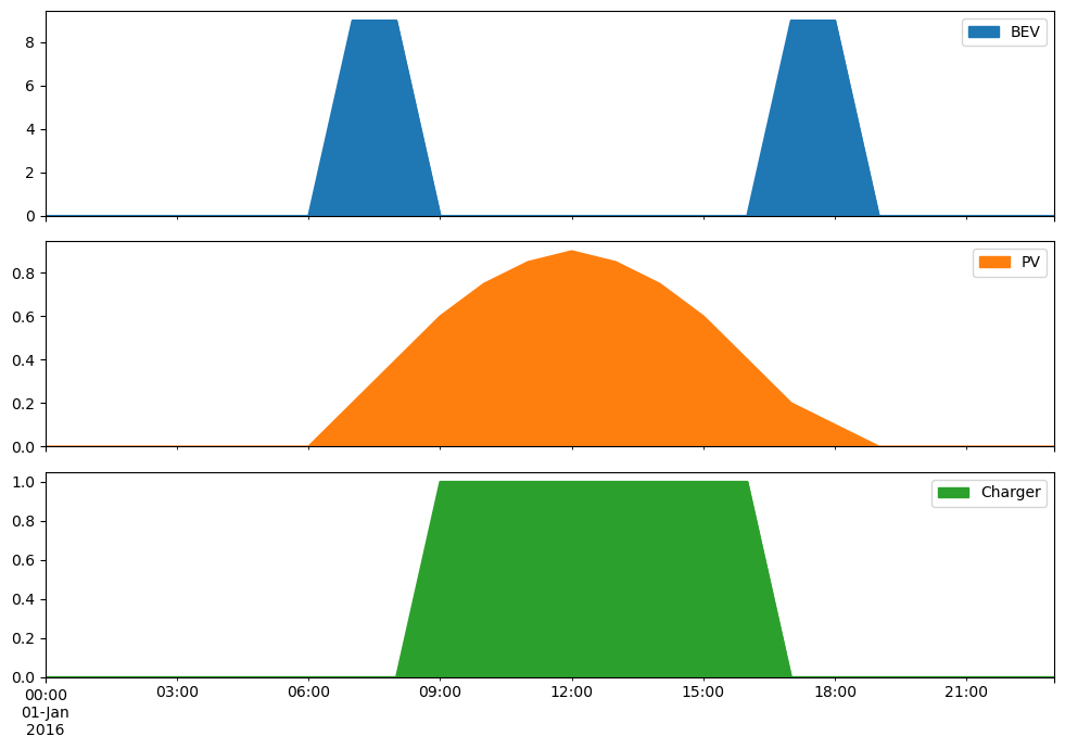
# use 24 hour period for consideration
index = pd.date_range("2016-01-01 00:00", "2016-01-01 23:00", freq="H")

# consumption pattern of BEV
bev_usage = pd.Series([0.0] * 7 + [9.0] * 2 + [0.0] * 8 + [9.0] * 2 + [0.0] * 5, index)

# solar PV panel generation per unit of capacity
pv_pu = pd.Series(
    [0.0] * 7
    + [0.2, 0.4, 0.6, 0.75, 0.85, 0.9, 0.85, 0.75, 0.6, 0.4, 0.2, 0.1]
    + [0.0] * 5,
    index,
)

# availability of charging - i.e. only when parked at office
charger_p_max_pu = pd.Series(0, index=index)
charger_p_max_pu["2016-01-01 09:00":"2016-01-01 16:00"] = 1.0
/tmp/ipykernel_3183/2212892536.py:2: FutureWarning: 'H' is deprecated and will be removed in a future version, please use 'h' instead.
  index = pd.date_range("2016-01-01 00:00", "2016-01-01 23:00", freq="H")
[3]:
df = pd.concat({"BEV": bev_usage, "PV": pv_pu, "Charger": charger_p_max_pu}, axis=1)
df.plot.area(subplots=True, figsize=(10, 7))
plt.tight_layout()
Initialize the network
[4]:
network = pypsa.Network()
network.set_snapshots(index)

network.add("Bus", "place of work", carrier="AC")

network.add("Bus", "battery", carrier="Li-ion")

network.add(
    "Generator",
    "PV panel",
    bus="place of work",
    p_nom_extendable=True,
    p_max_pu=pv_pu,
    capital_cost=1000.0,
)

network.add("Load", "driving", bus="battery", p_set=bev_usage)

network.add(
    "Link",
    "charger",
    bus0="place of work",
    bus1="battery",
    p_nom=120,  # super-charger with 120 kW
    p_max_pu=charger_p_max_pu,
    efficiency=0.9,
)


network.add("Store", "battery storage", bus="battery", e_cyclic=True, e_nom=100.0)
[5]:
network.optimize()
print("Objective:", network.objective)
INFO:linopy.model: Solve problem using Glpk solver
INFO:linopy.io: Writing time: 0.04s
INFO:linopy.solvers:GLPSOL--GLPK LP/MIP Solver 5.0
Parameter(s) specified in the command line:
 --lp /tmp/linopy-problem-eaey25px.lp --output /tmp/linopy-solve-9l01onss.sol
Reading problem data from '/tmp/linopy-problem-eaey25px.lp'...
217 rows, 97 columns, 325 non-zeros
1078 lines were read
GLPK Simplex Optimizer 5.0
217 rows, 97 columns, 325 non-zeros
Preprocessing...
48 rows, 49 columns, 104 non-zeros
Scaling...
 A: min|aij| =  4.000e-01  max|aij| =  1.000e+00  ratio =  2.500e+00
Problem data seem to be well scaled
Constructing initial basis...
Size of triangular part is 47
      0: obj =   0.000000000e+00 inf =   4.140e+02 (17)
      8: obj =   1.818181818e+04 inf =   0.000e+00 (0)
*    13: obj =   7.017543860e+03 inf =   0.000e+00 (0)
OPTIMAL LP SOLUTION FOUND
Time used:   0.0 secs
Memory used: 0.2 Mb (173076 bytes)
Writing basic solution to '/tmp/linopy-solve-9l01onss.sol'...

INFO:linopy.constants: Optimization successful:
Status: ok
Termination condition: optimal
Solution: 97 primals, 217 duals
Objective: 7.02e+03
Solver model: not available
Solver message: optimal

INFO:pypsa.optimization.optimize:The shadow-prices of the constraints Generator-ext-p-lower, Generator-ext-p-upper, Link-fix-p-lower, Link-fix-p-upper, Store-fix-e-lower, Store-fix-e-upper, Store-energy_balance were not assigned to the network.
Objective: 7017.54386
The optimal panel size in kW is
[6]:
network.generators.p_nom_opt["PV panel"]
[6]:
7.01754
[7]:
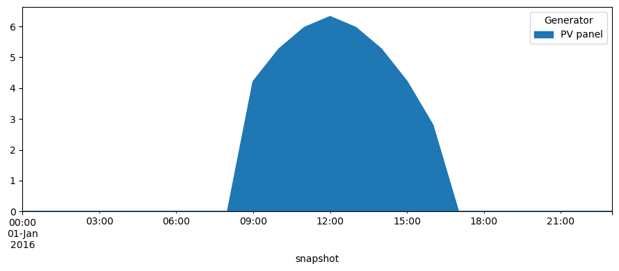
network.generators_t.p.plot.area(figsize=(9, 4))
plt.tight_layout()
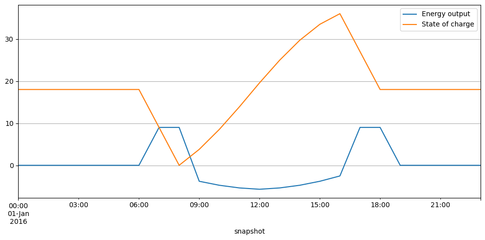
[8]:
df = pd.DataFrame(
    {attr: network.stores_t[attr]["battery storage"] for attr in ["p", "e"]}
)
df.plot(grid=True, figsize=(10, 5))
plt.legend(labels=["Energy output", "State of charge"])
plt.tight_layout()
The losses in kWh per pay are:
[9]:
(
    network.generators_t.p.loc[:, "PV panel"].sum()
    - network.loads_t.p.loc[:, "driving"].sum()
)
[9]:
4.000010000000003
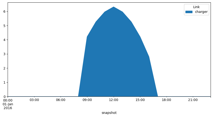
[10]:
network.links_t.p0.plot.area(figsize=(9, 5))
plt.tight_layout()