Battery Electric Vehicle Charging

In this example a battery electric vehicle (BEV) is driven 100 km in the morning and 100 km in the evening, to simulate commuting, and charged during the day by a solar panel at the driver’s place of work. The size of the panel is computed by the optimisation.

The BEV has a battery of size 100 kWh and an electricity consumption of 0.18 kWh/km.

NB: this example will use units of kW and kWh, unlike the PyPSA defaults

[1]:

import pypsa
import pandas as pd
import matplotlib.pyplot as plt

%matplotlib inline

[2]:

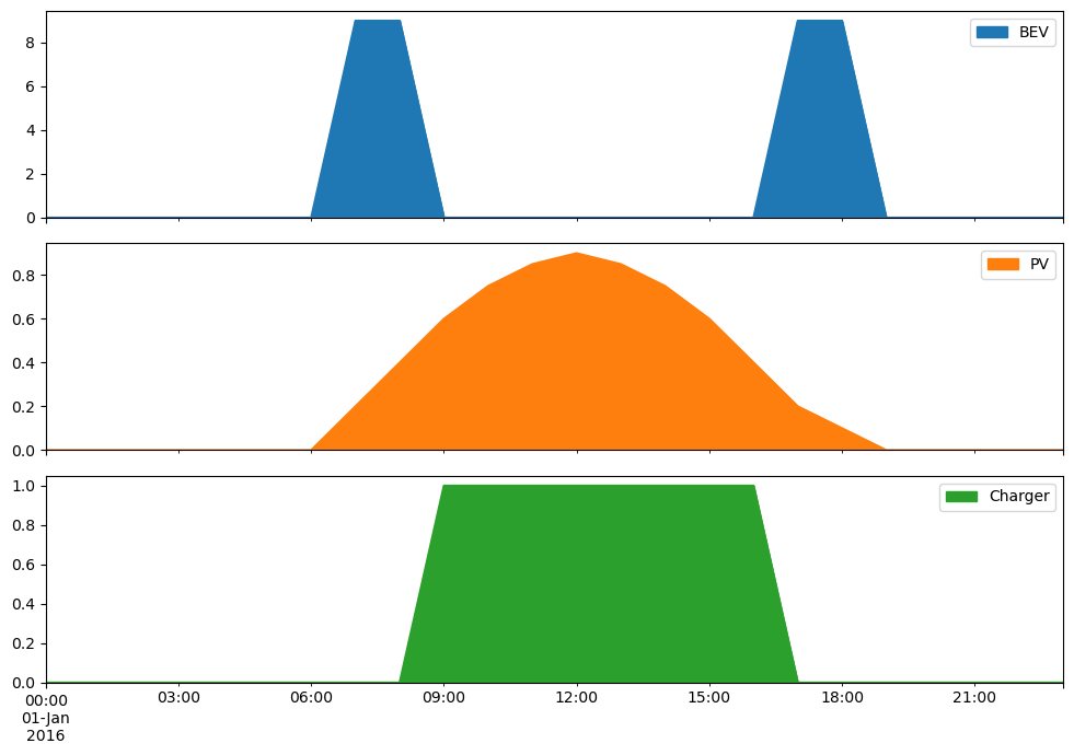
# use 24 hour period for consideration
index = pd.date_range("2016-01-01 00:00", "2016-01-01 23:00", freq="H")

# consumption pattern of BEV
bev_usage = pd.Series([0.0] * 7 + [9.0] * 2 + [0.0] * 8 + [9.0] * 2 + [0.0] * 5, index)

# solar PV panel generation per unit of capacity
pv_pu = pd.Series(
    [0.0] * 7
    + [0.2, 0.4, 0.6, 0.75, 0.85, 0.9, 0.85, 0.75, 0.6, 0.4, 0.2, 0.1]
    + [0.0] * 5,
    index,
)

# availability of charging - i.e. only when parked at office
charger_p_max_pu = pd.Series(0, index=index)
charger_p_max_pu["2016-01-01 09:00":"2016-01-01 16:00"] = 1.0

[3]:

df = pd.concat({"BEV": bev_usage, "PV": pv_pu, "Charger": charger_p_max_pu}, axis=1)
df.plot.area(subplots=True, figsize=(10, 7))
plt.tight_layout()

../_images/examples_battery-electric-vehicle-charging_3_0.png

Initialize the network

[4]:

network = pypsa.Network()
network.set_snapshots(index)

network.add("Bus", "place of work", carrier="AC")

network.add("Bus", "battery", carrier="Li-ion")

network.add(
    "Generator",
    "PV panel",
    bus="place of work",
    p_nom_extendable=True,
    p_max_pu=pv_pu,
    capital_cost=1000.0,
)

network.add("Load", "driving", bus="battery", p_set=bev_usage)

network.add(
    "Link",
    "charger",
    bus0="place of work",
    bus1="battery",
    p_nom=120,  # super-charger with 120 kW
    p_max_pu=charger_p_max_pu,
    efficiency=0.9,
)


network.add("Store", "battery storage", bus="battery", e_cyclic=True, e_nom=100.0)

[5]:

network.lopf()
print("Objective:", network.objective)

INFO:pypsa.linopf:Prepare linear problem
INFO:pypsa.linopf:Total preparation time: 0.11s
INFO:pypsa.linopf:Solve linear problem using Glpk solver
INFO:pypsa.linopf:Optimization successful. Objective value: 7.02e+03

Objective: 7017.54386

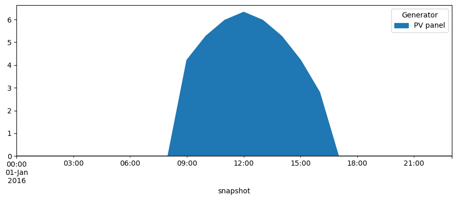
The optimal panel size in kW is

[6]:

network.generators.p_nom_opt["PV panel"]

[6]:

7.01754

[7]:

network.generators_t.p.plot.area(figsize=(9, 4))
plt.tight_layout()

../_images/examples_battery-electric-vehicle-charging_9_0.png

[8]:

df = pd.DataFrame(
    {attr: network.stores_t[attr]["battery storage"] for attr in ["p", "e"]}
)
df.plot(grid=True, figsize=(10, 5))
plt.legend(labels=["Energy output", "State of charge"])
plt.tight_layout()

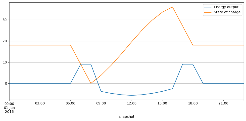
../_images/examples_battery-electric-vehicle-charging_10_0.png

The losses in kWh per pay are:

[9]:

(
    network.generators_t.p.loc[:, "PV panel"].sum()
    - network.loads_t.p.loc[:, "driving"].sum()
)

[9]:

4.000010000000003

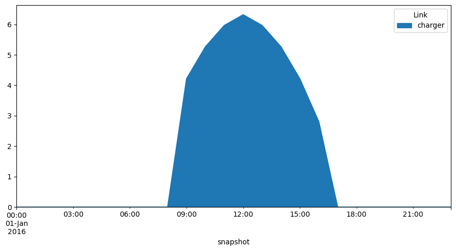
[10]:

network.links_t.p0.plot.area(figsize=(9, 5))
plt.tight_layout()

../_images/examples_battery-electric-vehicle-charging_13_0.png