Note
You can download this example as a Jupyter notebook or start it in interactive mode.
LOPF with coupling to heating sector
In this example three locations are optimised, each with an electric bus and a heating bus and corresponding loads. At each location the electric and heating buses are connected with heat pumps; heat can also be supplied to the heat bus with a boiler. The electric buses are connected with transmission lines and there are electrical generators at two of the nodes.
[1]:
import pypsa
import numpy as np
import pandas as pd
import matplotlib.pyplot as plt
import seaborn as sns

sns.set(rc={"figure.figsize": (9, 5)})
[2]:
network = pypsa.Network()
Add three buses of AC and heat carrier each
[3]:
for i in range(3):
    network.add("Bus", "electric bus {}".format(i), v_nom=20.0)
    network.add("Bus", "heat bus {}".format(i), carrier="heat")
network.buses
[3]:
| attribute | v_nom | type | x | y | carrier | unit | v_mag_pu_set | v_mag_pu_min | v_mag_pu_max | control | sub_network |
|---|---|---|---|---|---|---|---|---|---|---|---|
| Bus | |||||||||||
| electric bus 0 | 20.0 | 0.0 | 0.0 | AC | None | 1.0 | 0.0 | inf | PQ | ||
| heat bus 0 | 1.0 | 0.0 | 0.0 | heat | None | 1.0 | 0.0 | inf | PQ | ||
| electric bus 1 | 20.0 | 0.0 | 0.0 | AC | None | 1.0 | 0.0 | inf | PQ | ||
| heat bus 1 | 1.0 | 0.0 | 0.0 | heat | None | 1.0 | 0.0 | inf | PQ | ||
| electric bus 2 | 20.0 | 0.0 | 0.0 | AC | None | 1.0 | 0.0 | inf | PQ | ||
| heat bus 2 | 1.0 | 0.0 | 0.0 | heat | None | 1.0 | 0.0 | inf | PQ |
[4]:
network.buses["carrier"].value_counts()
[4]:
AC      3
heat    3
Name: carrier, dtype: int64
Add three lines in a ring
[5]:
for i in range(3):
    network.add(
        "Line",
        "line {}".format(i),
        bus0="electric bus {}".format(i),
        bus1="electric bus {}".format((i + 1) % 3),
        x=0.1,
        s_nom=1000,
    )
network.lines
[5]:
| attribute | bus0 | bus1 | type | x | r | g | b | s_nom | s_nom_extendable | s_nom_min | ... | v_ang_min | v_ang_max | sub_network | x_pu | r_pu | g_pu | b_pu | x_pu_eff | r_pu_eff | s_nom_opt |
|---|---|---|---|---|---|---|---|---|---|---|---|---|---|---|---|---|---|---|---|---|---|
| Line | |||||||||||||||||||||
| line 0 | electric bus 0 | electric bus 1 | 0.1 | 0.0 | 0.0 | 0.0 | 1000.0 | False | 0.0 | ... | -inf | inf | 0.0 | 0.0 | 0.0 | 0.0 | 0.0 | 0.0 | 0.0 | ||
| line 1 | electric bus 1 | electric bus 2 | 0.1 | 0.0 | 0.0 | 0.0 | 1000.0 | False | 0.0 | ... | -inf | inf | 0.0 | 0.0 | 0.0 | 0.0 | 0.0 | 0.0 | 0.0 | ||
| line 2 | electric bus 2 | electric bus 0 | 0.1 | 0.0 | 0.0 | 0.0 | 1000.0 | False | 0.0 | ... | -inf | inf | 0.0 | 0.0 | 0.0 | 0.0 | 0.0 | 0.0 | 0.0 |
3 rows × 29 columns
Connect the electric to the heat buses with heat pumps with COP 3
[6]:
for i in range(3):
    network.add(
        "Link",
        "heat pump {}".format(i),
        bus0="electric bus {}".format(i),
        bus1="heat bus {}".format(i),
        p_nom=100,
        efficiency=3.0,
    )
network.links
[6]:
| attribute | bus0 | bus1 | type | carrier | efficiency | build_year | lifetime | p_nom | p_nom_extendable | p_nom_min | ... | p_set | p_min_pu | p_max_pu | capital_cost | marginal_cost | length | terrain_factor | ramp_limit_up | ramp_limit_down | p_nom_opt |
|---|---|---|---|---|---|---|---|---|---|---|---|---|---|---|---|---|---|---|---|---|---|
| Link | |||||||||||||||||||||
| heat pump 0 | electric bus 0 | heat bus 0 | 3.0 | 0 | inf | 100.0 | False | 0.0 | ... | 0.0 | 0.0 | 1.0 | 0.0 | 0.0 | 0.0 | 1.0 | NaN | NaN | 0.0 | ||
| heat pump 1 | electric bus 1 | heat bus 1 | 3.0 | 0 | inf | 100.0 | False | 0.0 | ... | 0.0 | 0.0 | 1.0 | 0.0 | 0.0 | 0.0 | 1.0 | NaN | NaN | 0.0 | ||
| heat pump 2 | electric bus 2 | heat bus 2 | 3.0 | 0 | inf | 100.0 | False | 0.0 | ... | 0.0 | 0.0 | 1.0 | 0.0 | 0.0 | 0.0 | 1.0 | NaN | NaN | 0.0 |
3 rows × 21 columns
Add carriers
[7]:
network.add("Carrier", "gas", co2_emissions=0.27)
network.add("Carrier", "biomass", co2_emissions=0.0)
network.carriers
[7]:
| attribute | co2_emissions | color | nice_name | max_growth |
|---|---|---|---|---|
| Carrier | ||||
| gas | 0.27 | inf | ||
| biomass | 0.00 | inf |
Add a gas generator at bus 0, a biomass generator at bus 1 and a boiler at all heat buses
[8]:
network.add(
    "Generator",
    "gas generator",
    bus="electric bus 0",
    p_nom=100,
    marginal_cost=50,
    carrier="gas",
    efficiency=0.3,
)

network.add(
    "Generator",
    "biomass generator",
    bus="electric bus 1",
    p_nom=100,
    marginal_cost=100,
    efficiency=0.3,
    carrier="biomass",
)

for i in range(3):
    network.add(
        "Generator",
        "boiler {}".format(i),
        bus="heat bus {}".format(i),
        p_nom=1000,
        efficiency=0.9,
        marginal_cost=20.0,
        carrier="gas",
    )

network.generators
[8]:
| attribute | bus | control | type | p_nom | p_nom_extendable | p_nom_min | p_nom_max | p_min_pu | p_max_pu | p_set | ... | shut_down_cost | min_up_time | min_down_time | up_time_before | down_time_before | ramp_limit_up | ramp_limit_down | ramp_limit_start_up | ramp_limit_shut_down | p_nom_opt |
|---|---|---|---|---|---|---|---|---|---|---|---|---|---|---|---|---|---|---|---|---|---|
| Generator | |||||||||||||||||||||
| gas generator | electric bus 0 | PQ | 100.0 | False | 0.0 | inf | 0.0 | 1.0 | 0.0 | ... | 0.0 | 0 | 0 | 1 | 0 | NaN | NaN | 1.0 | 1.0 | 0.0 | |
| biomass generator | electric bus 1 | PQ | 100.0 | False | 0.0 | inf | 0.0 | 1.0 | 0.0 | ... | 0.0 | 0 | 0 | 1 | 0 | NaN | NaN | 1.0 | 1.0 | 0.0 | |
| boiler 0 | heat bus 0 | PQ | 1000.0 | False | 0.0 | inf | 0.0 | 1.0 | 0.0 | ... | 0.0 | 0 | 0 | 1 | 0 | NaN | NaN | 1.0 | 1.0 | 0.0 | |
| boiler 1 | heat bus 1 | PQ | 1000.0 | False | 0.0 | inf | 0.0 | 1.0 | 0.0 | ... | 0.0 | 0 | 0 | 1 | 0 | NaN | NaN | 1.0 | 1.0 | 0.0 | |
| boiler 2 | heat bus 2 | PQ | 1000.0 | False | 0.0 | inf | 0.0 | 1.0 | 0.0 | ... | 0.0 | 0 | 0 | 1 | 0 | NaN | NaN | 1.0 | 1.0 | 0.0 |
5 rows × 30 columns
Add electric loads and heat loads.
[9]:
for i in range(3):
    network.add(
        "Load",
        "electric load {}".format(i),
        bus="electric bus {}".format(i),
        p_set=i * 10,
    )

for i in range(3):
    network.add(
        "Load",
        "heat load {}".format(i),
        bus="heat bus {}".format(i),
        p_set=(3 - i) * 10,
    )

network.loads
[9]:
| attribute | bus | carrier | type | p_set | q_set | sign |
|---|---|---|---|---|---|---|
| Load | ||||||
| electric load 0 | electric bus 0 | 0.0 | 0.0 | -1.0 | ||
| electric load 1 | electric bus 1 | 10.0 | 0.0 | -1.0 | ||
| electric load 2 | electric bus 2 | 20.0 | 0.0 | -1.0 | ||
| heat load 0 | heat bus 0 | 30.0 | 0.0 | -1.0 | ||
| heat load 1 | heat bus 1 | 20.0 | 0.0 | -1.0 | ||
| heat load 2 | heat bus 2 | 10.0 | 0.0 | -1.0 |
We define a function for the LOPF
[10]:
def run_lopf():
    network.lopf()
    df = pd.concat(
        [
            network.generators_t.p.loc["now"],
            network.links_t.p0.loc["now"],
            network.loads_t.p.loc["now"],
        ],
        keys=["Generators", "Links", "Line"],
        names=["Component", "index"],
    ).reset_index(name="Production")

    sns.barplot(data=df, x="index", y="Production", hue="Component")
    plt.title(f"Objective: {network.objective}")
    plt.xticks(rotation=90)
    plt.tight_layout()
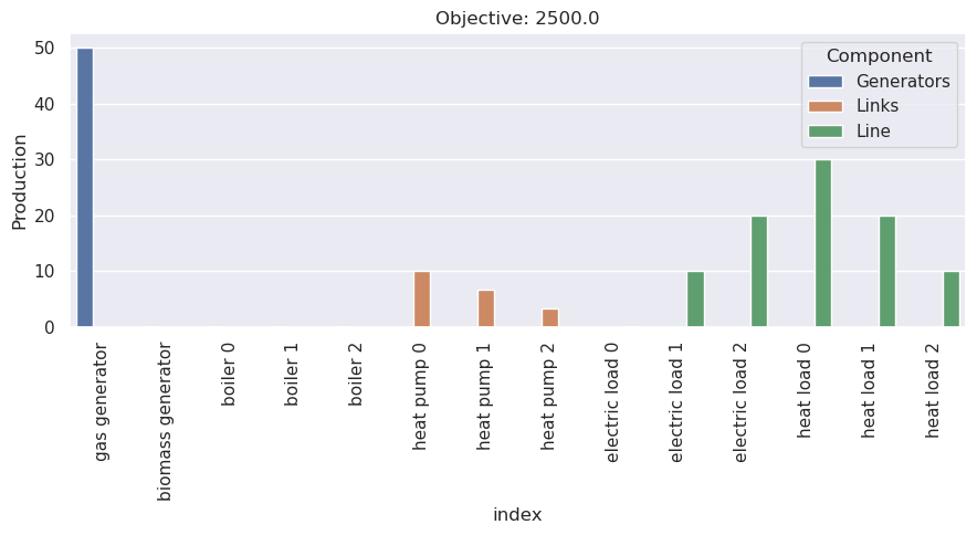
[11]:
run_lopf()
INFO:pypsa.linopf:Prepare linear problem
INFO:pypsa.linopf:Total preparation time: 0.15s
INFO:pypsa.linopf:Solve linear problem using Glpk solver
INFO:pypsa.linopf:Optimization successful. Objective value: 2.50e+03
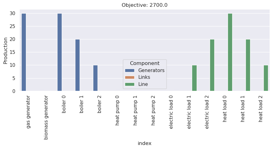
Now, rerun with marginal costs for the heat pump operation.
[12]:
network.links.marginal_cost = 10
run_lopf()
INFO:pypsa.linopf:Prepare linear problem
INFO:pypsa.linopf:Total preparation time: 0.15s
INFO:pypsa.linopf:Solve linear problem using Glpk solver
INFO:pypsa.linopf:Optimization successful. Objective value: 2.70e+03
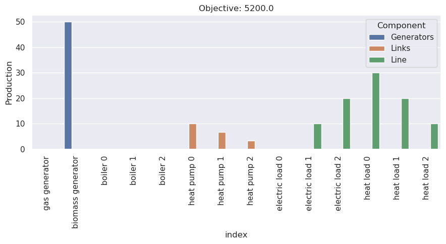
Finally, rerun with no CO2 emissions.
[13]:
network.add("GlobalConstraint", "co2_limit", sense="<=", constant=0.0)

run_lopf()
INFO:pypsa.linopf:Prepare linear problem
INFO:pypsa.linopf:Total preparation time: 0.17s
INFO:pypsa.linopf:Solve linear problem using Glpk solver
INFO:pypsa.linopf:Optimization successful. Objective value: 5.20e+03