Note

You can download this example as a Jupyter notebook or start it in interactive mode.

Network Clustering

In this example, we show how pypsa can deal with spatial clustering of networks.

import pypsa
import re
import numpy as np
import matplotlib.pyplot as plt
import cartopy.crs as ccrs
import pandas as pd
from pypsa.networkclustering import get_clustering_from_busmap, busmap_by_kmeans

n = pypsa.examples.scigrid_de()
n.lines["type"] = np.nan  # delete the 'type' specifications to make this example easier

WARNING:pypsa.io:Importing network from PyPSA version v0.17.1 while current version is v0.21.3. Read the release notes at https://pypsa.readthedocs.io/en/latest/release_notes.html to prepare your network for import.
INFO:pypsa.io:Imported network scigrid-de.nc has buses, generators, lines, loads, storage_units, transformers

The important information that pypsa needs for spatial clustering is in the busmap. It contains the mapping of which buses should be grouped together, similar to the groupby groups as we know it from pandas.

You can either calculate a busmap from the provided clustering algorithms or you can create/use your own busmap.

Cluster by custom busmap

Let’s start with creating our own. In the following, we group all buses together which belong to the same operator. Buses which do not have a specific operator just stay on its own.

groups = n.buses.operator.apply(lambda x: re.split(" |,|;", x)[0])
busmap = groups.where(groups != "", n.buses.index)

Now we cluster the network based on the busmap.

C = get_clustering_from_busmap(n, busmap)

C is a Clustering object which contains all important information. Among others, the new network is now stored in that Clustering object.

nc = C.network

We have a look at the original and the clustered topology

fig, (ax, ax1) = plt.subplots(
    1, 2, subplot_kw={"projection": ccrs.EqualEarth()}, figsize=(12, 12)
)
plot_kwrgs = dict(bus_sizes=1e-3, line_widths=0.5)
n.plot(ax=ax, title="original", **plot_kwrgs)
nc.plot(ax=ax1, title="clustered by operator", **plot_kwrgs)
fig.tight_layout()

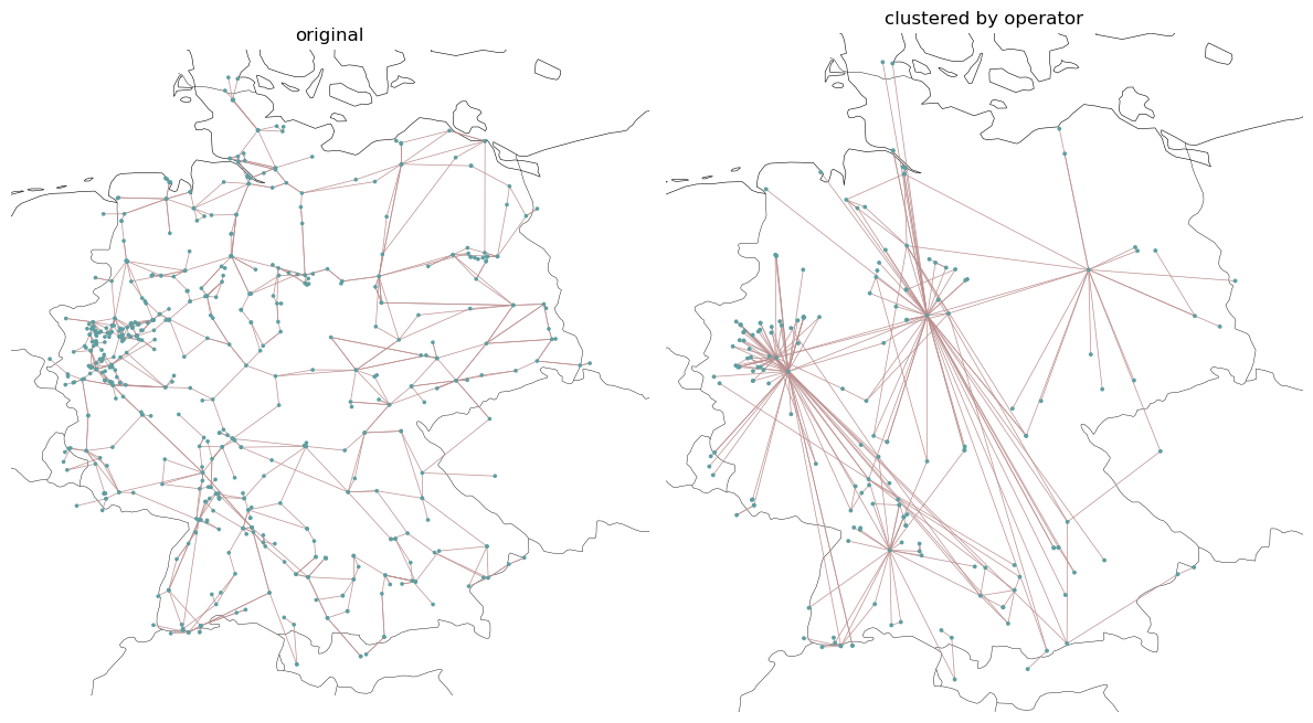
Looks a bit messy as over 120 buses do not have assigned operators.

Clustering by busmap created from K-means

Let’s now make a clustering based on the kmeans algorithm. Therefore we calculate the busmap from a non-weighted kmeans clustering.

weighting = pd.Series(1, n.buses.index)
busmap2 = busmap_by_kmeans(n, bus_weightings=weighting, n_clusters=50)

/home/docs/checkouts/readthedocs.org/user_builds/pypsa/conda/v0.21.3/lib/python3.11/site-packages/sklearn/cluster/_kmeans.py:870: FutureWarning: The default value of `n_init` will change from 10 to 'auto' in 1.4. Set the value of `n_init` explicitly to suppress the warning
  warnings.warn(

We use this new kmeans-based busmap to create a new clustered method.

C2 = get_clustering_from_busmap(n, busmap2)
nc2 = C2.network

Again, let’s plot the networks to compare:

fig, (ax, ax1) = plt.subplots(
    1, 2, subplot_kw={"projection": ccrs.EqualEarth()}, figsize=(12, 12)
)
plot_kwrgs = dict(bus_sizes=1e-3, line_widths=0.5)
n.plot(ax=ax, title="original", **plot_kwrgs)
nc2.plot(ax=ax1, title="clustered by kmeans", **plot_kwrgs)
fig.tight_layout()

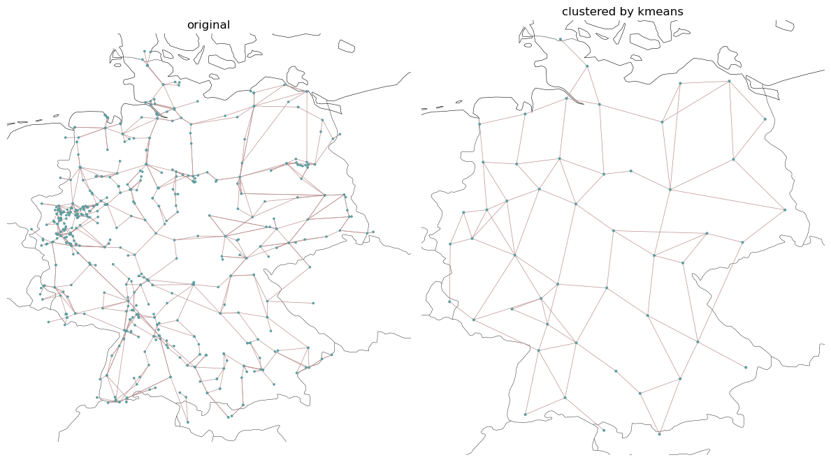
There are other clustering algorithms in the pipeline of pypsa as the hierarchical clustering which performs better than the kmeans. Also the get_clustering_from_busmap function supports various arguments on how components in the network should be aggregated.