Note
You can download this example as a Jupyter notebook or start it in interactive mode.
Screening curve analysis
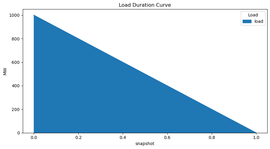
Compute the long-term equilibrium power plant investment for a given load duration curve (1000-1000z for z \(\in\) [0,1]) and a given set of generator investment options.
[1]:
import pypsa
import numpy as np
import pandas as pd
import matplotlib.pyplot as plt

%matplotlib inline
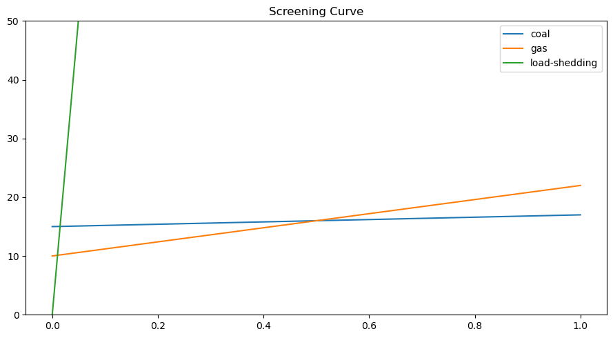
Generator marginal (m) and capital (c) costs in EUR/MWh - numbers chosen for simple answer.
[2]:
generators = {
    "coal": {"m": 2, "c": 15},
    "gas": {"m": 12, "c": 10},
    "load-shedding": {"m": 1012, "c": 0},
}
The screening curve intersections are at 0.01 and 0.5.
[3]:
x = np.linspace(0, 1, 101)
df = pd.DataFrame(
    {key: pd.Series(item["c"] + x * item["m"], x) for key, item in generators.items()}
)
df.plot(ylim=[0, 50], title="Screening Curve", figsize=(9, 5))
plt.tight_layout()
[4]:
n = pypsa.Network()

num_snapshots = 1001
n.snapshots = np.linspace(0, 1, num_snapshots)
n.snapshot_weightings = n.snapshot_weightings / num_snapshots

n.add("Bus", name="bus")

n.add("Load", name="load", bus="bus", p_set=1000 - 1000 * n.snapshots.values)

for gen in generators:
    n.add(
        "Generator",
        name=gen,
        bus="bus",
        p_nom_extendable=True,
        marginal_cost=float(generators[gen]["m"]),
        capital_cost=float(generators[gen]["c"]),
    )
[5]:
n.loads_t.p_set.plot.area(title="Load Duration Curve", figsize=(9, 5), ylabel="MW")
plt.tight_layout()
[6]:
n.lopf(solver_name="cbc")
n.objective
INFO:pypsa.linopf:Prepare linear problem
INFO:pypsa.linopf:Total preparation time: 0.14s
INFO:pypsa.linopf:Solve linear problem using Cbc solver
INFO:pypsa.linopf:Optimization successful. Objective value: 1.47e+04
[6]:
14706.191555
The capacity is set by total electricity required.
NB: No load shedding since all prices are below 10 000.
[7]:
n.generators.p_nom_opt.round(2)
[7]:
Generator
coal             500
gas              490
load-shedding     10
Name: p_nom_opt, dtype: int64
[8]:
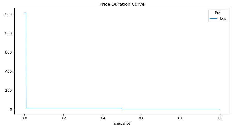
n.buses_t.marginal_price.plot(title="Price Duration Curve", figsize=(9, 4))
plt.tight_layout()
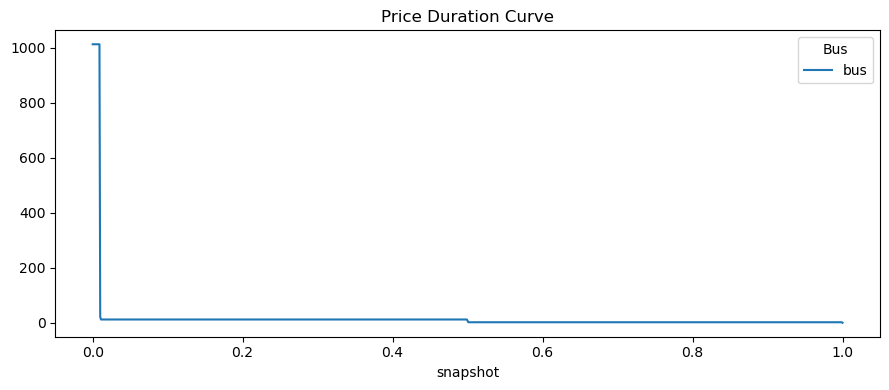
The prices correspond either to VOLL (1012) for first 0.01 or the marginal costs (12 for 0.49 and 2 for 0.5)
Except for (infinitesimally small) points at the screening curve intersections, which correspond to changing the load duration near the intersection, so that capacity changes. This explains 7 = (12+10 - 15) (replacing coal with gas) and 22 = (12+10) (replacing load-shedding with gas).
Note: What remains unclear is what is causing :nbsphinx-math:`l `= 0… it should be 2.
[9]:
n.buses_t.marginal_price.round(2).sum(axis=1).value_counts()
[9]:
2.0       499
12.0      489
1012.0     10
22.0        1
7.0         1
0.0         1
dtype: int64
[10]:
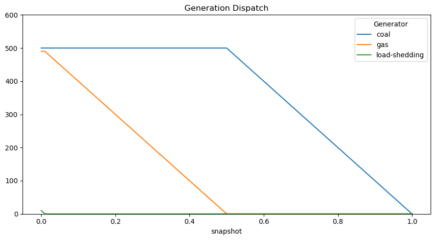
n.generators_t.p.plot(ylim=[0, 600], title="Generation Dispatch", figsize=(9, 5))
plt.tight_layout()
Demonstrate zero-profit condition.
The total cost is given by
[11]:
(
    n.generators.p_nom_opt * n.generators.capital_cost
    + n.generators_t.p.multiply(n.snapshot_weightings.generators, axis=0).sum()
    * n.generators.marginal_cost
)
[11]:
Generator
coal             8249.750250
gas              6400.839161
load-shedding      55.604396
dtype: float64
The total revenue by
[12]:
(
    n.generators_t.p.multiply(n.snapshot_weightings.generators, axis=0)
    .multiply(n.buses_t.marginal_price["bus"], axis=0)
    .sum(0)
)
[12]:
Generator
coal             8249.749500
gas              6400.837660
load-shedding      55.604395
dtype: float64
Now, take the capacities from the above long-term equilibrium, then disallow expansion.
Show that the resulting market prices are identical.
This holds in this example, but does NOT necessarily hold and breaks down in some circumstances (for example, when there is a lot of storage and inter-temporal shifting).
[13]:
n.generators.p_nom_extendable = False
n.generators.p_nom = n.generators.p_nom_opt
[14]:
n.lopf();
INFO:pypsa.linopf:Prepare linear problem
INFO:pypsa.linopf:Total preparation time: 0.12s
INFO:pypsa.linopf:Solve linear problem using Glpk solver
INFO:pypsa.linopf:Optimization successful. Objective value: 2.31e+03
/home/docs/checkouts/readthedocs.org/user_builds/pypsa/conda/v0.21.1/lib/python3.10/site-packages/pypsa/linopf.py:1173: FutureWarning: In a future version, `df.iloc[:, i] = newvals` will attempt to set the values inplace instead of always setting a new array. To retain the old behavior, use either `df[df.columns[i]] = newvals` or, if columns are non-unique, `df.isetitem(i, newvals)`
  pnl[attr].loc[sns, df.columns] = df
[15]:
n.buses_t.marginal_price.plot(title="Price Duration Curve", figsize=(9, 5))
plt.tight_layout()
[16]:
n.buses_t.marginal_price.sum(axis=1).value_counts()
[16]:
1.999998       500
11.999988      490
1012.000990     10
0.000000         1
dtype: int64
Demonstrate zero-profit condition. Differences are due to singular times, see above, not a problem
Total costs
[17]:
(
    n.generators.p_nom * n.generators.capital_cost
    + n.generators_t.p.multiply(n.snapshot_weightings.generators, axis=0).sum()
    * n.generators.marginal_cost
)
[17]:
Generator
coal             8249.750250
gas              6400.839161
load-shedding      55.604396
dtype: float64
Total revenue
[18]:
(
    n.generators_t.p.multiply(n.snapshot_weightings.generators, axis=0)
    .multiply(n.buses_t.marginal_price["bus"], axis=0)
    .sum()
)
[18]:
Generator
coal             8242.25950
gas              6395.94746
load-shedding      55.60445
dtype: float64