Note
You can download this example as a Jupyter notebook or start it in interactive mode.
Non-linear power flow after LOPF
In this example, the dispatch of generators is optimised using the linear OPF, then a non-linear power flow is run on the resulting dispatch.
Data sources
Grid: based on SciGRID Version 0.2 which is based on OpenStreetMap.
Load size and location: based on Landkreise (NUTS 3) GDP and population.
Load time series: from ENTSO-E hourly data, scaled up uniformly by factor 1.12 (a simplification of the methodology in Schumacher, Hirth (2015)).
Conventional power plant capacities and locations: BNetzA list.
Wind and solar capacities and locations: EEG Stammdaten, based on http://www.energymap.info/download.html, which represents capacities at the end of 2014. Units without PLZ are removed.
Wind and solar time series: REatlas, Andresen et al, “Validation of Danish wind time series from a new global renewable energy atlas for energy system analysis,” Energy 93 (2015) 1074 - 1088.
Where SciGRID nodes have been split into 220kV and 380kV substations, all load and generation is attached to the 220kV substation.
Warnings
The data behind the notebook is no longer supported. See https://github.com/PyPSA/pypsa-eur for a newer model that covers the whole of Europe.
This dataset is ONLY intended to demonstrate the capabilities of PyPSA and is NOT (yet) accurate enough to be used for research purposes.
Known problems include:
Rough approximations have been made for missing grid data, e.g. 220kV-380kV transformers and connections between close sub-stations missing from OSM.
There appears to be some unexpected congestion in parts of the network, which may mean for example that the load attachment method (by Voronoi cell overlap with Landkreise) isn’t working, particularly in regions with a high density of substations.
Attaching power plants to the nearest high voltage substation may not reflect reality.
There is no proper n-1 security in the calculations - this can either be simulated with a blanket e.g. 70% reduction in thermal limits (as done here) or a proper security constrained OPF (see e.g. http://www.pypsa.org/examples/scigrid-sclopf.ipynb).
The borders and neighbouring countries are not represented.
Hydroelectric power stations are not modelled accurately.
The marginal costs are illustrative, not accurate.
Only the first day of 2011 is in the github dataset, which is not representative. The full year of 2011 can be downloaded at http://www.pypsa.org/examples/scigrid-with-load-gen-trafos-2011.zip.
The ENTSO-E total load for Germany may not be scaled correctly; it is scaled up uniformly by factor 1.12 (a simplification of the methodology in Schumacher, Hirth (2015), which suggests monthly factors).
Biomass from the EEG Stammdaten are not read in at the moment.
Power plant start up costs, ramping limits/costs, minimum loading rates are not considered.
[1]:
import pypsa
import numpy as np
import pandas as pd
import os
import matplotlib.pyplot as plt
import cartopy.crs as ccrs

%matplotlib inline
[2]:
network = pypsa.examples.scigrid_de(from_master=True)
WARNING:pypsa.io:Importing network from PyPSA version v0.17.1 while current version is v0.21.1. Read the release notes at https://pypsa.readthedocs.io/en/latest/release_notes.html to prepare your network for import.
INFO:pypsa.io:Imported network scigrid-de.nc has buses, generators, lines, loads, storage_units, transformers
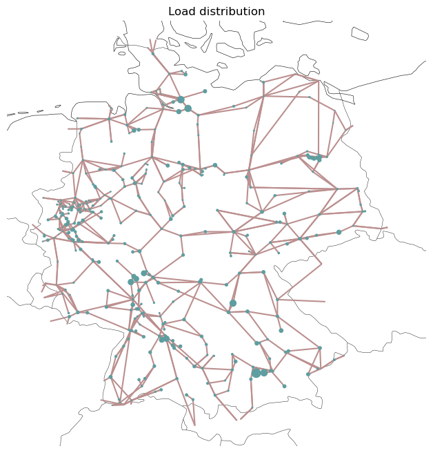
Plot the distribution of the load and of generating tech
[3]:
fig, ax = plt.subplots(
    1, 1, subplot_kw={"projection": ccrs.EqualEarth()}, figsize=(8, 8)
)

load_distribution = (
    network.loads_t.p_set.loc[network.snapshots[0]].groupby(network.loads.bus).sum()
)
network.plot(bus_sizes=1e-5 * load_distribution, ax=ax, title="Load distribution");
[4]:
network.generators.groupby("carrier")["p_nom"].sum()
[4]:
carrier
Brown Coal       20879.500000
Gas              23913.130000
Geothermal          31.700000
Hard Coal        25312.600000
Multiple           152.700000
Nuclear          12068.000000
Oil               2710.200000
Other             3027.800000
Run of River      3999.100000
Solar            37041.524779
Storage Hydro     1445.000000
Waste             1645.900000
Wind Offshore     2973.500000
Wind Onshore     37339.895329
Name: p_nom, dtype: float64
[5]:
network.storage_units.groupby("carrier")["p_nom"].sum()
[5]:
carrier
Pumped Hydro    9179.5
Name: p_nom, dtype: float64
[6]:
techs = ["Gas", "Brown Coal", "Hard Coal", "Wind Offshore", "Wind Onshore", "Solar"]

n_graphs = len(techs)
n_cols = 3
if n_graphs % n_cols == 0:
    n_rows = n_graphs // n_cols
else:
    n_rows = n_graphs // n_cols + 1


fig, axes = plt.subplots(
    nrows=n_rows, ncols=n_cols, subplot_kw={"projection": ccrs.EqualEarth()}
)
size = 6
fig.set_size_inches(size * n_cols, size * n_rows)

for i, tech in enumerate(techs):
    i_row = i // n_cols
    i_col = i % n_cols

    ax = axes[i_row, i_col]
    gens = network.generators[network.generators.carrier == tech]
    gen_distribution = (
        gens.groupby("bus").sum()["p_nom"].reindex(network.buses.index, fill_value=0.0)
    )
    network.plot(ax=ax, bus_sizes=2e-5 * gen_distribution)
    ax.set_title(tech)
fig.tight_layout()
/tmp/ipykernel_4364/3986438909.py:24: FutureWarning: The default value of numeric_only in DataFrameGroupBy.sum is deprecated. In a future version, numeric_only will default to False. Either specify numeric_only or select only columns which should be valid for the function.
  gens.groupby("bus").sum()["p_nom"].reindex(network.buses.index, fill_value=0.0)
Run Linear Optimal Power Flow on the first day of 2011.
To approximate n-1 security and allow room for reactive power flows, don’t allow any line to be loaded above 70% of their thermal rating
[7]:
contingency_factor = 0.7
network.lines.s_max_pu = contingency_factor
There are some infeasibilities without small extensions
[8]:
network.lines.loc[["316", "527", "602"], "s_nom"] = 1715
We performing a linear OPF for one day, 4 snapshots at a time.
[9]:
group_size = 4
network.storage_units.state_of_charge_initial = 0.0

for i in range(int(24 / group_size)):
    # set the initial state of charge based on previous round
    if i:
        network.storage_units.state_of_charge_initial = (
            network.storage_units_t.state_of_charge.loc[
                network.snapshots[group_size * i - 1]
            ]
        )
    network.lopf(
        network.snapshots[group_size * i : group_size * i + group_size],
        solver_name="cbc",
        pyomo=False,
    )
INFO:pypsa.linopf:Prepare linear problem
INFO:pypsa.linopf:Total preparation time: 1.28s
INFO:pypsa.linopf:Solve linear problem using Cbc solver
INFO:pypsa.linopf:Optimization successful. Objective value: 1.45e+06
INFO:pypsa.linopf:Prepare linear problem
INFO:pypsa.linopf:Total preparation time: 1.28s
INFO:pypsa.linopf:Solve linear problem using Cbc solver
INFO:pypsa.linopf:Optimization successful. Objective value: 8.74e+05
INFO:pypsa.linopf:Prepare linear problem
INFO:pypsa.linopf:Total preparation time: 1.27s
INFO:pypsa.linopf:Solve linear problem using Cbc solver
INFO:pypsa.linopf:Optimization successful. Objective value: 7.91e+05
INFO:pypsa.linopf:Prepare linear problem
INFO:pypsa.linopf:Total preparation time: 1.27s
INFO:pypsa.linopf:Solve linear problem using Cbc solver
INFO:pypsa.linopf:Optimization successful. Objective value: 1.46e+06
INFO:pypsa.linopf:Prepare linear problem
INFO:pypsa.linopf:Total preparation time: 1.26s
INFO:pypsa.linopf:Solve linear problem using Cbc solver
INFO:pypsa.linopf:Optimization successful. Objective value: 2.65e+06
INFO:pypsa.linopf:Prepare linear problem
INFO:pypsa.linopf:Total preparation time: 1.27s
INFO:pypsa.linopf:Solve linear problem using Cbc solver
INFO:pypsa.linopf:Optimization successful. Objective value: 2.14e+06
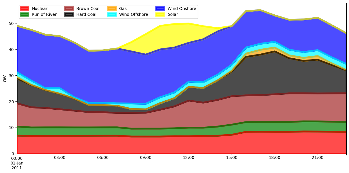
[10]:
p_by_carrier = network.generators_t.p.groupby(network.generators.carrier, axis=1).sum()
p_by_carrier.drop(
    (p_by_carrier.max()[p_by_carrier.max() < 1700.0]).index, axis=1, inplace=True
)
p_by_carrier.columns
[10]:
Index(['Brown Coal', 'Gas', 'Hard Coal', 'Nuclear', 'Run of River', 'Solar',
       'Wind Offshore', 'Wind Onshore'],
      dtype='object', name='carrier')
[11]:
colors = {
    "Brown Coal": "brown",
    "Hard Coal": "k",
    "Nuclear": "r",
    "Run of River": "green",
    "Wind Onshore": "blue",
    "Solar": "yellow",
    "Wind Offshore": "cyan",
    "Waste": "orange",
    "Gas": "orange",
}
# reorder
cols = [
    "Nuclear",
    "Run of River",
    "Brown Coal",
    "Hard Coal",
    "Gas",
    "Wind Offshore",
    "Wind Onshore",
    "Solar",
]
p_by_carrier = p_by_carrier[cols]
[12]:
c = [colors[col] for col in p_by_carrier.columns]

fig, ax = plt.subplots(figsize=(12, 6))
(p_by_carrier / 1e3).plot(kind="area", ax=ax, linewidth=4, color=c, alpha=0.7)
ax.legend(ncol=4, loc="upper left")
ax.set_ylabel("GW")
ax.set_xlabel("")
fig.tight_layout()
[13]:
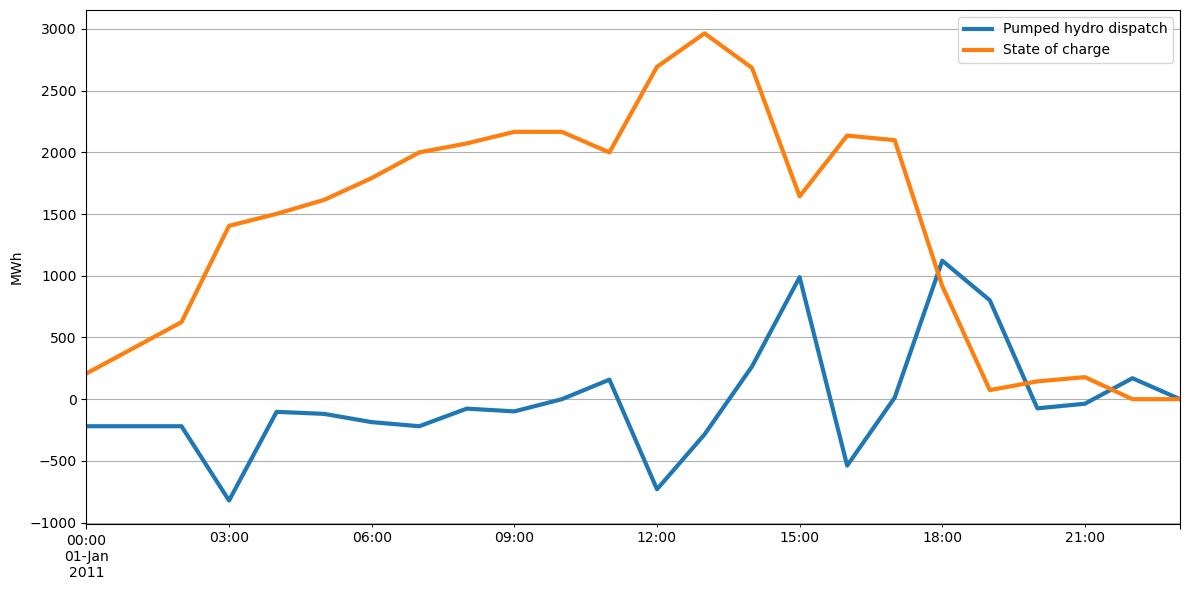
fig, ax = plt.subplots(figsize=(12, 6))

p_storage = network.storage_units_t.p.sum(axis=1)
state_of_charge = network.storage_units_t.state_of_charge.sum(axis=1)
p_storage.plot(label="Pumped hydro dispatch", ax=ax, linewidth=3)
state_of_charge.plot(label="State of charge", ax=ax, linewidth=3)

ax.legend()
ax.grid()
ax.set_ylabel("MWh")
ax.set_xlabel("")
fig.tight_layout()
[14]:
now = network.snapshots[4]
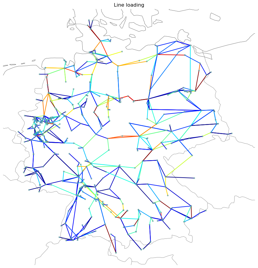
With the linear load flow, there is the following per unit loading:
[15]:
loading = network.lines_t.p0.loc[now] / network.lines.s_nom
loading.describe()
[15]:
count    852.000000
mean      -0.002892
std        0.258607
min       -0.700000
25%       -0.129688
50%        0.003084
75%        0.122643
max        0.700000
dtype: float64
[16]:
fig, ax = plt.subplots(subplot_kw={"projection": ccrs.EqualEarth()}, figsize=(9, 9))
network.plot(
    ax=ax,
    line_colors=abs(loading),
    line_cmap=plt.cm.jet,
    title="Line loading",
    bus_sizes=1e-3,
    bus_alpha=0.7,
)
fig.tight_layout();
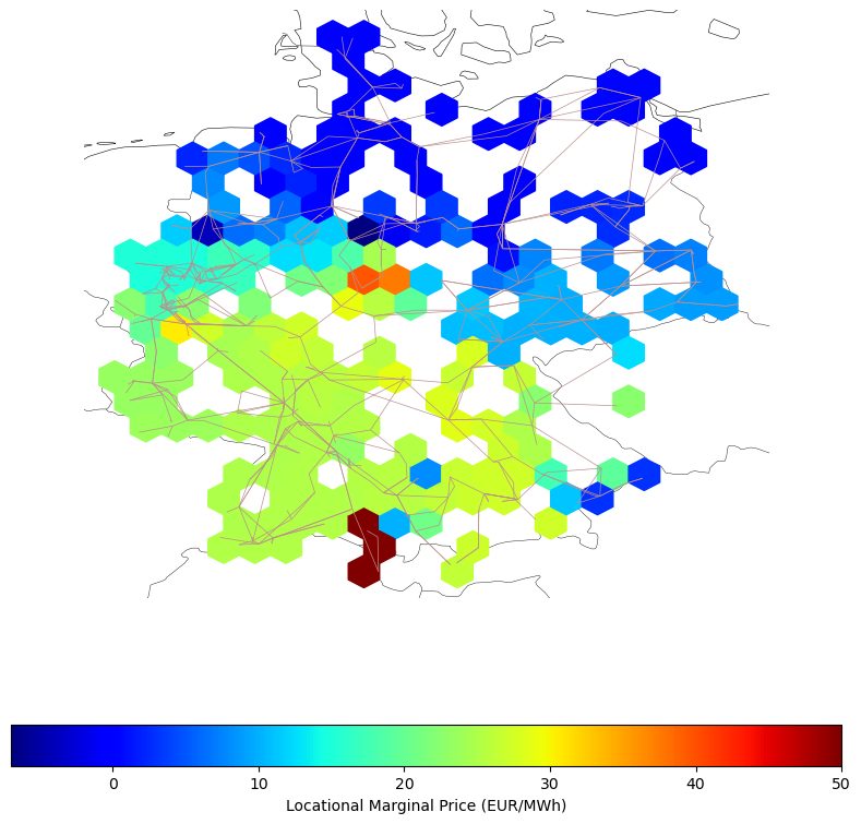
Let’s have a look at the marginal prices
[17]:
network.buses_t.marginal_price.loc[now].describe()
[17]:
count    585.000000
mean      15.737598
std       10.941994
min      -10.397824
25%        6.992120
50%       15.841191
75%       25.048186
max       52.150119
Name: 2011-01-01 04:00:00, dtype: float64
[18]:
fig, ax = plt.subplots(subplot_kw={"projection": ccrs.PlateCarree()}, figsize=(8, 8))

plt.hexbin(
    network.buses.x,
    network.buses.y,
    gridsize=20,
    C=network.buses_t.marginal_price.loc[now],
    cmap=plt.cm.jet,
    zorder=3,
)
network.plot(ax=ax, line_widths=pd.Series(0.5, network.lines.index), bus_sizes=0)

cb = plt.colorbar(location="bottom")
cb.set_label("Locational Marginal Price (EUR/MWh)")
fig.tight_layout()
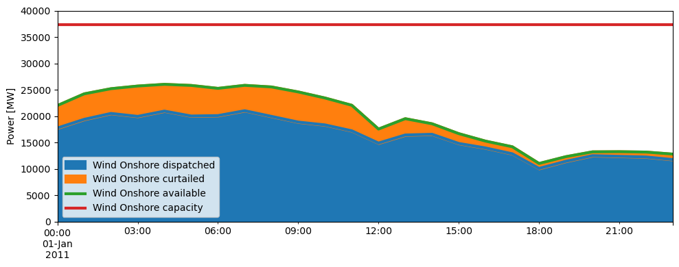
Curtailment variable
By considering how much power is available and how much is generated, you can see what share is curtailed:
[19]:
carrier = "Wind Onshore"

capacity = network.generators.groupby("carrier").sum().at[carrier, "p_nom"]
p_available = network.generators_t.p_max_pu.multiply(network.generators["p_nom"])
p_available_by_carrier = p_available.groupby(network.generators.carrier, axis=1).sum()
p_curtailed_by_carrier = p_available_by_carrier - p_by_carrier
/tmp/ipykernel_4364/2097778438.py:3: FutureWarning: The default value of numeric_only in DataFrameGroupBy.sum is deprecated. In a future version, numeric_only will default to False. Either specify numeric_only or select only columns which should be valid for the function.
  capacity = network.generators.groupby("carrier").sum().at[carrier, "p_nom"]
[20]:
p_df = pd.DataFrame(
    {
        carrier + " available": p_available_by_carrier[carrier],
        carrier + " dispatched": p_by_carrier[carrier],
        carrier + " curtailed": p_curtailed_by_carrier[carrier],
    }
)

p_df[carrier + " capacity"] = capacity
[21]:
p_df["Wind Onshore curtailed"][p_df["Wind Onshore curtailed"] < 0.0] = 0.0
[22]:
fig, ax = plt.subplots(figsize=(10, 4))
p_df[[carrier + " dispatched", carrier + " curtailed"]].plot(
    kind="area", ax=ax, linewidth=3
)
p_df[[carrier + " available", carrier + " capacity"]].plot(ax=ax, linewidth=3)

ax.set_xlabel("")
ax.set_ylabel("Power [MW]")
ax.set_ylim([0, 40000])
ax.legend()
fig.tight_layout()
Non-Linear Power Flow
Now perform a full Newton-Raphson power flow on the first hour. For the PF, set the P to the optimised P.
[23]:
network.generators_t.p_set = network.generators_t.p
network.storage_units_t.p_set = network.storage_units_t.p
Set all buses to PV, since we don’t know what Q set points are
[24]:
network.generators.control = "PV"

# Need some PQ buses so that Jacobian doesn't break
f = network.generators[network.generators.bus == "492"]
network.generators.loc[f.index, "control"] = "PQ"
Now, perform the non-linear PF.
[25]:
info = network.pf();
INFO:pypsa.pf:Performing non-linear load-flow on AC sub-network SubNetwork 0 for snapshots DatetimeIndex(['2011-01-01 00:00:00', '2011-01-01 01:00:00',
               '2011-01-01 02:00:00', '2011-01-01 03:00:00',
               '2011-01-01 04:00:00', '2011-01-01 05:00:00',
               '2011-01-01 06:00:00', '2011-01-01 07:00:00',
               '2011-01-01 08:00:00', '2011-01-01 09:00:00',
               '2011-01-01 10:00:00', '2011-01-01 11:00:00',
               '2011-01-01 12:00:00', '2011-01-01 13:00:00',
               '2011-01-01 14:00:00', '2011-01-01 15:00:00',
               '2011-01-01 16:00:00', '2011-01-01 17:00:00',
               '2011-01-01 18:00:00', '2011-01-01 19:00:00',
               '2011-01-01 20:00:00', '2011-01-01 21:00:00',
               '2011-01-01 22:00:00', '2011-01-01 23:00:00'],
              dtype='datetime64[ns]', name='snapshot', freq=None)
/home/docs/checkouts/readthedocs.org/user_builds/pypsa/conda/v0.21.1/lib/python3.10/site-packages/pypsa/pf.py:107: FutureWarning: In a future version, `df.iloc[:, i] = newvals` will attempt to set the values inplace instead of always setting a new array. To retain the old behavior, use either `df[df.columns[i]] = newvals` or, if columns are non-unique, `df.isetitem(i, newvals)`
  network.buses_t[n].loc[snapshots, buses_o] = sum(
INFO:pypsa.pf:Newton-Raphson solved in 4 iterations with error of 0.000000 in 0.043035 seconds
INFO:pypsa.pf:Newton-Raphson solved in 4 iterations with error of 0.000000 in 0.040724 seconds
INFO:pypsa.pf:Newton-Raphson solved in 4 iterations with error of 0.000000 in 0.040150 seconds
INFO:pypsa.pf:Newton-Raphson solved in 4 iterations with error of 0.000000 in 0.040566 seconds
INFO:pypsa.pf:Newton-Raphson solved in 4 iterations with error of 0.000000 in 0.040491 seconds
INFO:pypsa.pf:Newton-Raphson solved in 4 iterations with error of 0.000000 in 0.040657 seconds
INFO:pypsa.pf:Newton-Raphson solved in 4 iterations with error of 0.000000 in 0.041343 seconds
INFO:pypsa.pf:Newton-Raphson solved in 4 iterations with error of 0.000000 in 0.040733 seconds
INFO:pypsa.pf:Newton-Raphson solved in 4 iterations with error of 0.000000 in 0.040972 seconds
INFO:pypsa.pf:Newton-Raphson solved in 4 iterations with error of 0.000000 in 0.040727 seconds
INFO:pypsa.pf:Newton-Raphson solved in 4 iterations with error of 0.000000 in 0.041167 seconds
INFO:pypsa.pf:Newton-Raphson solved in 4 iterations with error of 0.000000 in 0.040925 seconds
INFO:pypsa.pf:Newton-Raphson solved in 4 iterations with error of 0.000000 in 0.041304 seconds
INFO:pypsa.pf:Newton-Raphson solved in 4 iterations with error of 0.000000 in 0.040739 seconds
INFO:pypsa.pf:Newton-Raphson solved in 4 iterations with error of 0.000000 in 0.041206 seconds
INFO:pypsa.pf:Newton-Raphson solved in 4 iterations with error of 0.000000 in 0.042044 seconds
INFO:pypsa.pf:Newton-Raphson solved in 4 iterations with error of 0.000000 in 0.041972 seconds
INFO:pypsa.pf:Newton-Raphson solved in 4 iterations with error of 0.000000 in 0.041063 seconds
INFO:pypsa.pf:Newton-Raphson solved in 4 iterations with error of 0.000000 in 0.041233 seconds
INFO:pypsa.pf:Newton-Raphson solved in 4 iterations with error of 0.000000 in 0.041802 seconds
INFO:pypsa.pf:Newton-Raphson solved in 4 iterations with error of 0.000000 in 0.040929 seconds
INFO:pypsa.pf:Newton-Raphson solved in 4 iterations with error of 0.000000 in 0.040781 seconds
INFO:pypsa.pf:Newton-Raphson solved in 4 iterations with error of 0.000000 in 0.040827 seconds
INFO:pypsa.pf:Newton-Raphson solved in 4 iterations with error of 0.000000 in 0.042031 seconds
Any failed to converge?
[26]:
(~info.converged).any().any()
[26]:
False
With the non-linear load flow, there is the following per unit loading of the full thermal rating.
[27]:
(network.lines_t.p0.loc[now] / network.lines.s_nom).describe()
[27]:
count    852.000000
mean       0.000435
std        0.260958
min       -0.813382
25%       -0.125478
50%        0.003032
75%        0.126690
max        0.827203
dtype: float64
Let’s inspect the voltage angle differences across the lines have (in degrees)
[28]:
df = network.lines.copy()

for b in ["bus0", "bus1"]:
    df = pd.merge(
        df, network.buses_t.v_ang.loc[[now]].T, how="left", left_on=b, right_index=True
    )

s = df[str(now) + "_x"] - df[str(now) + "_y"]

(s * 180 / np.pi).describe()
[28]:
count    852.000000
mean      -0.022968
std        2.373832
min      -12.158420
25%       -0.462981
50%        0.001586
75%        0.537448
max       17.959258
dtype: float64
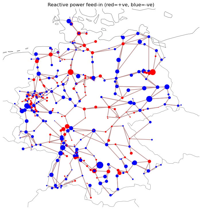
Plot the reactive power
[29]:
fig, ax = plt.subplots(subplot_kw={"projection": ccrs.EqualEarth()}, figsize=(9, 9))

q = network.buses_t.q.loc[now]
bus_colors = pd.Series("r", network.buses.index)
bus_colors[q < 0.0] = "b"

network.plot(
    bus_sizes=1e-4 * abs(q),
    ax=ax,
    bus_colors=bus_colors,
    title="Reactive power feed-in (red=+ve, blue=-ve)",
);