Note

You can download this example as a Jupyter notebook or start it in interactive mode.

Redispatch Example with SciGRID network

In this example, we compare a 2-stage market with an initial market clearing in two bidding zones with flow-based market coupling and a subsequent redispatch market (incl. curtailment) to an idealised nodal pricing scheme.

import pypsa
import matplotlib.pyplot as plt
import cartopy.crs as ccrs
from pypsa.descriptors import get_switchable_as_dense as as_dense

solver = "cbc"

Load example network

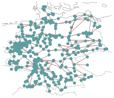
o = pypsa.examples.scigrid_de(from_master=True)
o.lines.s_max_pu = 0.7
o.lines.loc[["316", "527", "602"], "s_nom"] = 1715
o.set_snapshots([o.snapshots[12]])

WARNING:pypsa.io:Importing network from PyPSA version v0.17.1 while current version is v0.21.1. Read the release notes at https://pypsa.readthedocs.io/en/latest/release_notes.html to prepare your network for import.
INFO:pypsa.io:Imported network scigrid-de.nc has buses, generators, lines, loads, storage_units, transformers

n = o.copy()  # for redispatch model
m = o.copy()  # for market model

o.plot();

Solve original nodal market model o

First, let us solve a nodal market using the original model o:

o.lopf(solver_name=solver, pyomo=False)

INFO:pypsa.linopf:Prepare linear problem
INFO:pypsa.linopf:Total preparation time: 1.22s
INFO:pypsa.linopf:Solve linear problem using Cbc solver
INFO:pypsa.linopf:Optimization successful. Objective value: 3.01e+05

('ok', 'optimal')

Costs are 301 k€.

Build market model m with two bidding zones

For this example, we split the German transmission network into two market zones at latitude 51 degrees.

You can build any other market zones by providing an alternative mapping from bus to zone.

zones = (n.buses.y > 51).map(lambda x: "North" if x else "South")

Next, we assign this mapping to the market model m.

We re-assign the buses of all generators and loads, and remove all transmission lines within each bidding zone.

Here, we assume that the bidding zones are coupled through the transmission lines that connect them.

for c in m.iterate_components(m.one_port_components):
    c.df.bus = c.df.bus.map(zones)

for c in m.iterate_components(m.branch_components):
    c.df.bus0 = c.df.bus0.map(zones)
    c.df.bus1 = c.df.bus1.map(zones)
    internal = c.df.bus0 == c.df.bus1
    m.mremove(c.name, c.df.loc[internal].index)

m.mremove("Bus", m.buses.index)
m.madd("Bus", ["North", "South"]);

Now, we can solve the coupled market with two bidding zones.

m.lopf(solver_name=solver, pyomo=False)

INFO:pypsa.linopf:Prepare linear problem
INFO:pypsa.linopf:Total preparation time: 0.22s
INFO:pypsa.linopf:Solve linear problem using Cbc solver
INFO:pypsa.linopf:Optimization successful. Objective value: 2.14e+05

('ok', 'optimal')

Costs are 214 k€, which is much lower than the 301 k€ of the nodal market.

This is because network restrictions apart from the North/South division are not taken into account yet.

We can look at the market clearing prices of each zone:

m.buses_t.marginal_price

Bus	North	South
snapshot
2011-01-01 12:00:00	8.0	25.0

Build redispatch model n

Next, based on the market outcome with two bidding zones m, we build a secondary redispatch market n that rectifies transmission constraints through curtailment and ramping up/down thermal generators.

First, we fix the dispatch of generators to the results from the market simulation. (For simplicity, this example disregards storage units.)

p = m.generators_t.p / m.generators.p_nom
n.generators_t.p_min_pu = p
n.generators_t.p_max_pu = p

Then, we add generators bidding into redispatch market using the following assumptions:

• All generators can reduce their dispatch to zero. This includes also curtailment of renewables.

• All generators can increase their dispatch to their available/nominal capacity.

• No changes to the marginal costs, i.e. reducing dispatch lowers costs.

With these settings, the 2-stage market should result in the same cost as the nodal market.

g_up = n.generators.copy()
g_down = n.generators.copy()

g_up.index = g_up.index.map(lambda x: x + " ramp up")
g_down.index = g_down.index.map(lambda x: x + " ramp down")

up = (
    as_dense(m, "Generator", "p_max_pu") * m.generators.p_nom - m.generators_t.p
).clip(0) / m.generators.p_nom
down = -m.generators_t.p / m.generators.p_nom

up.columns = up.columns.map(lambda x: x + " ramp up")
down.columns = down.columns.map(lambda x: x + " ramp down")

n.madd("Generator", g_up.index, p_max_pu=up, **g_up.drop("p_max_pu", axis=1))

n.madd(
    "Generator",
    g_down.index,
    p_min_pu=down,
    p_max_pu=0,
    **g_down.drop(["p_max_pu", "p_min_pu"], axis=1)
);

Now, let’s solve the redispatch market:

n.lopf(solver_name=solver, pyomo=False)

INFO:pypsa.linopf:Prepare linear problem
INFO:pypsa.linopf:Total preparation time: 1.54s
INFO:pypsa.linopf:Solve linear problem using Cbc solver
INFO:pypsa.linopf:Optimization successful. Objective value: 3.01e+05

('ok', 'optimal')

And, as expected, the costs are the same as for the nodal market: 301 k€.

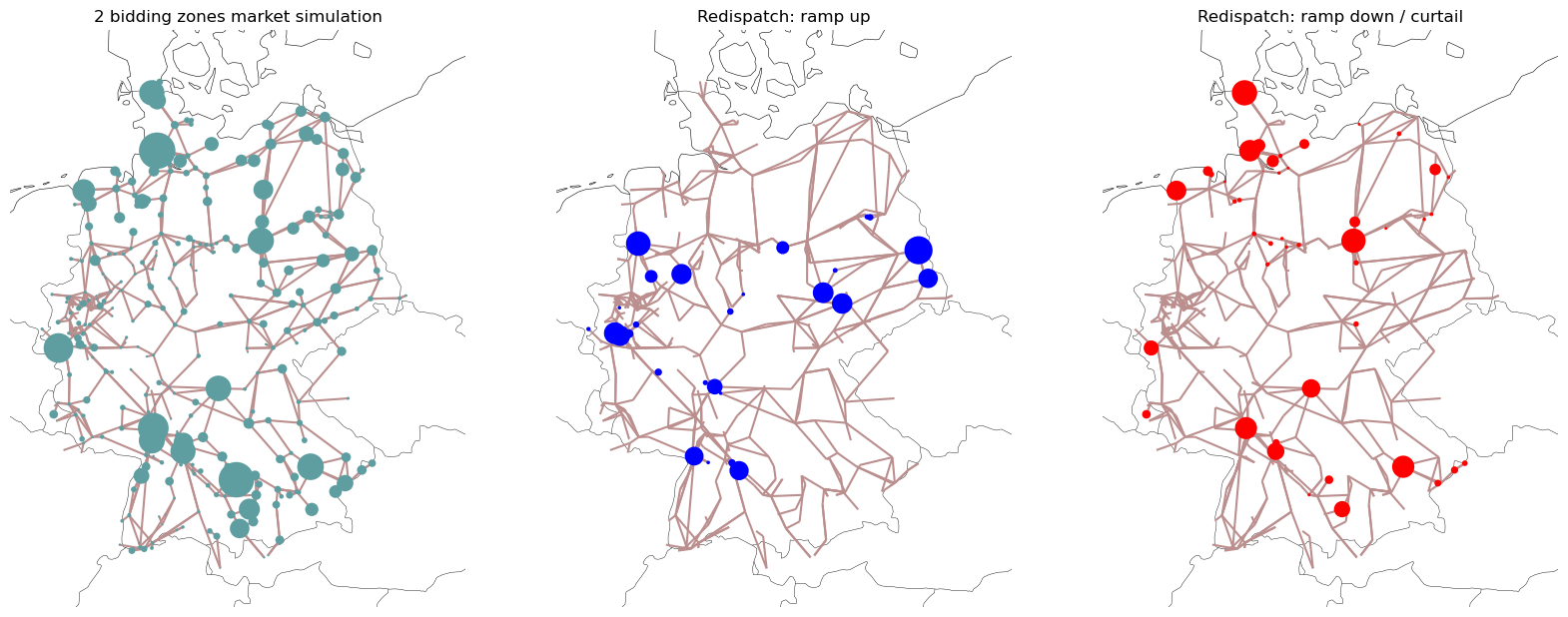
Now, we can plot both the market results of the 2 bidding zone market and the redispatch results:

fig, axs = plt.subplots(
    1, 3, figsize=(20, 10), subplot_kw={"projection": ccrs.AlbersEqualArea()}
)

market = (
    n.generators_t.p[m.generators.index]
    .T.squeeze()
    .groupby(n.generators.bus)
    .sum()
    .div(2e4)
)
n.plot(ax=axs[0], bus_sizes=market, title="2 bidding zones market simulation")

redispatch_up = (
    n.generators_t.p.filter(like="ramp up")
    .T.squeeze()
    .groupby(n.generators.bus)
    .sum()
    .div(2e4)
)
n.plot(
    ax=axs[1], bus_sizes=redispatch_up, bus_colors="blue", title="Redispatch: ramp up"
)

redispatch_down = (
    n.generators_t.p.filter(like="ramp down")
    .T.squeeze()
    .groupby(n.generators.bus)
    .sum()
    .div(-2e4)
)
n.plot(
    ax=axs[2],
    bus_sizes=redispatch_down,
    bus_colors="red",
    title="Redispatch: ramp down / curtail",
);

We can also read out the final dispatch of each generator:

grouper = n.generators.index.str.split(" ramp", expand=True).get_level_values(0)

n.generators_t.p.groupby(grouper, axis=1).sum().squeeze()

1 Gas                     0.000000
1 Hard Coal               0.000000
1 Solar                  11.326192
1 Wind Onshore            1.754744
100_220kV Solar          14.913326
                           ...
98 Wind Onshore          71.451646
99_220kV Gas              0.000000
99_220kV Hard Coal        0.000000
99_220kV Solar            8.246606
99_220kV Wind Onshore     3.432939
Name: 2011-01-01 12:00:00, Length: 1423, dtype: float64

Changing bidding strategies in redispatch market

We can also formulate other bidding strategies or compensation mechanisms for the redispatch market.

For example, that ramping up a generator is twice as expensive.

n.generators.loc[n.generators.index.str.contains("ramp up"), "marginal_cost"] *= 2

Or that generators need to be compensated for curtailing them or ramping them down at 50% of their marginal cost.

n.generators.loc[n.generators.index.str.contains("ramp down"), "marginal_cost"] *= -0.5

In this way, the outcome should be more expensive than the ideal nodal market:

n.lopf(solver_name=solver, pyomo=False)

INFO:pypsa.linopf:Prepare linear problem
INFO:pypsa.linopf:Total preparation time: 1.51s
INFO:pypsa.linopf:Solve linear problem using Cbc solver
INFO:pypsa.linopf:Optimization successful. Objective value: 5.59e+05

('ok', 'optimal')

Costs are now 559 k€ compared to 301 k€.