Components#
PyPSA represents the power system using the following components:
component |
list_name |
description |
type |
|---|---|---|---|
Network |
networks |
Container for all components and functions which act upon the whole network. |
|
SubNetwork |
sub_networks |
Subsets of buses and passive branches (i.e. lines and transformers) that are connected (i.e. synchronous areas). |
|
Bus |
buses |
Electrically fundamental node where x-port objects attach. |
|
Carrier |
carriers |
Energy carrier, such as AC, DC, heat, wind, PV or coal. Buses have direct carriers and Generators indicate their primary energy carriers. The Carrier can track properties relevant for global constraints, such as CO2 emissions. |
|
GlobalConstraint |
global_constraints |
Constraints for OPF that affect many components, such as CO2 emission constraints. |
|
Line |
lines |
Lines include distribution and transmission lines, overhead lines and cables. |
passive_branch |
LineType |
line_types |
Standard line types with per length values for impedances. |
standard_type |
Transformer |
transformers |
2-winding transformer. |
passive_branch |
TransformerType |
transformer_types |
Standard 2-winding transformer types. |
standard_type |
Link |
links |
Link between two buses with controllable active power - can be used for a transport power flow model OR as a simplified version of point-to-point DC connection OR as a lossy energy converter. NB: for a lossless bi-directional HVDC or transport link, set p_min_pu = -1 and efficiency = 1. NB: It is assumed that the links neither produce nor consume reactive power. |
controllable_branch |
Load |
loads |
PQ power consumer. |
controllable_one_port |
Generator |
generators |
Power generator. |
controllable_one_port |
StorageUnit |
storage_units |
Storage unit with fixed nominal-energy-to-nominal-power ratio. |
controllable_one_port |
Store |
stores |
Generic store, whose capacity may be optimised. |
controllable_one_port |
ShuntImpedance |
shunt_impedances |
Shunt y = g + jb. |
passive_one_port |
Shape |
shapes |
Geographical shapes of the network components. |
shape |
This table is also available as a dictionary within each network
object as network.components.
For each class of components, the data describing the components is
stored in a pandas.DataFrame corresponding to the
list_name. For example, all static data for buses is stored in
network.buses. In this pandas.DataFrame the index corresponds
to the unique string names of the components, while the columns
correspond to the component static attributes. For example,
network.buses.v_nom gives the nominal voltages of each bus.
Time-varying series attributes are stored in a dictionary of
pandas.DataFrame based on the list_name followed by _t,
e.g. network.buses_t. For example, the set points for the per unit
voltage magnitude at each bus for each snapshot can be found in
network.buses_t.v_mag_pu_set. Please also read Time-varying data.
For each component class their attributes, their types
(float/boolean/string/int/series), their defaults, their descriptions
and their statuses are stored in a pandas.DataFrame in the
dictionary network.components as
e.g. network.components["Bus"]["attrs"]. This data is reproduced
as tables for each component below.
Their status is either “Input” for those which the user specifies or “Output” for those results which PyPSA calculates.
The inputs can be either “required”, if the user must give the input, or “optional”, if PyPSA will use a sensible default if the user gives no input.
For functions such as Power Flow and Power System Optimization the inputs used and outputs given are listed in their documentation.
Network#
The Network is the overall container for all components. It also
has the major functions as methods, such as network.optimize() and
network.pf().
attribute |
type |
unit |
default |
description |
status |
|---|---|---|---|---|---|
name |
string |
n/a |
n/a |
Unique name |
Input (required) |
snapshots |
list or pandas.Index |
n/a |
[“now”] |
List of snapshots or time steps. All time-dependent series quantities are indexed by |
Input (optional) |
snapshot_weightings |
pandas.DataFrame |
hours |
1 |
The weightings applied to each snapshot, so that snapshots can represent more than one hour or fractions of one hour. The objective weightings are used to weight snapshots in the LOPF objective function. The store weightings determine the state of charge change for stores and storage units. The generator weightings are used when calculating global constraints. |
Input (optional) |
investment_periods |
pandas.Index |
years |
[] |
Time periods of investment. Only used for multi investment optimisation. Years have to be integer and increasing (e.g. [2025,2030,2035]). Default is an empty pd.Index([]). |
Input (optional) |
investment_period_weightings |
pandas.DataFrame |
n/a |
1 |
Weightings applied to each investment period. Objective weightings are multiplied with all cost coefficients in the objective function of the respective investment period (e.g. used to include social discount rate). Years weighting denote the elapsed time until the subsequent investment period (e.g. used for global constraints CO2 emissions). |
Input (optional) |
now |
any |
n/a |
“now” |
The current snapshot/time/scenario, relevant e.g. when |
Input (optional) |
srid |
integer |
n/a |
4326 |
Spatial Reference System Indentifier for x,y coordinates of buses. It defaults to standard longitude and latitude. |
Input (optional) |
crs |
CRS-like |
n/a |
n/a |
Coordinate Reference System for the Shape components. It defaults to standard longitude and latitude, given in srid. |
Input (optional) |
buses |
pandas.DataFrame |
n/a |
n/a |
All static bus information compiled by PyPSA from inputs. Index is bus names, columns are bus attributes. |
Output |
buses_t |
dictionary of pandas.DataFrames |
n/a |
n/a |
All time-dependent bus information compiled by PyPSA from inputs. Dictionary keys are time-dependent series attributes, index is network.snapshots, columns are bus names. |
Output |
lines |
pandas.DataFrame |
n/a |
n/a |
All static line information compiled by PyPSA from inputs. Index is line names, columns are line attributes. |
Output |
lines_t |
dictionary of pandas.DataFrames |
n/a |
n/a |
All time-dependent line information compiled by PyPSA from inputs. Dictionary keys are time-dependent series attributes, index is network.snapshots, columns are line names. |
Output |
components |
pandas.DataFrame |
n/a |
n/a |
For each component type (buses, lines, etc.): static component information compiled by PyPSA from inputs. Index is component names, columns are component attributes. |
Output |
components_t |
dictionary of pandas.DataFrames |
n/a |
n/a |
For each component type (buses, lines, etc.): time-dependent component information compiled by PyPSA from inputs. Dictionary keys are time-dependent series attributes, index is network.snapshots, columns are component names. |
Output |
branches() |
pandas.DataFrame |
n/a |
n/a |
Dynamically generated concatenation of branch DataFrames: network.lines, network.transformers and network.links. Note that this is a copy and therefore changing entries will NOT update the original. |
Output |
graph() |
networkx. OrderedMultiGraph |
n/a |
n/a |
Graph of network. |
Output |
Sub-Network#
Sub-networks are determined by PyPSA and should not be entered by the user.
Sub-networks are subsets of buses and passive branches (i.e. lines and transformers) that are connected.
They have a uniform energy carrier inherited from the buses, such as
“DC”, “AC”, “heat” or “gas”. In the case of “AC” sub-networks, these
correspond to synchronous areas. Only “AC” and “DC” sub-networks can
contain passive branches; all other sub-networks must contain a single
isolated bus.
The power flow in sub-networks is determined by the passive flow through passive branches due to the impedances of the passive branches.
Sub-Network are determined by calling
network.determine_network_topology().
attribute |
type |
unit |
default |
description |
status |
|---|---|---|---|---|---|
name |
string |
n/a |
n/a |
Unique name based on order of sub-network in list of sub-networks. |
Output |
carrier |
string |
n/a |
AC |
Energy carrier: could be for example “AC” or “DC” (for electrical networks) or “gas” or “heat”. The carrier is determined from the buses in sub_network. |
Output |
slack_bus |
string |
n/a |
n/a |
Name of slack bus. |
Output |
Bus#
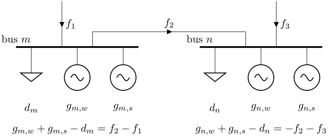
The bus is the fundamental node of the network, to which components like loads, generators and transmission lines attach. It enforces energy conservation for all elements feeding in and out of it (i.e. like Kirchhoff’s Current Law).
attribute |
type |
unit |
default |
description |
status |
|---|---|---|---|---|---|
name |
string |
n/a |
n/a |
Unique name |
Input (required) |
v_nom |
float |
kV |
1 |
Nominal voltage |
Input (optional) |
type |
string |
n/a |
n/a |
Placeholder for bus type. Not yet implemented. |
Input (optional) |
x |
float |
n/a |
0 |
Position (e.g. longitude); the Spatial Reference System Identifier (SRID) is set in network.srid. |
Input (optional) |
y |
float |
n/a |
0 |
Position (e.g. latitude); the Spatial Reference System Identifier (SRID) is set in network.srid. |
Input (optional) |
carrier |
string |
n/a |
AC |
Energy carrier: can be “AC” or “DC” for electrical buses, or “heat” or “gas”. |
Input (optional) |
unit |
string |
n/a |
None |
Unit of the bus’ carrier if the implicitly assumed unit (“MW”) is inappropriate (e.g. “t/h”, “MWh_th/h”). Only descriptive. Does not influence any PyPSA functions. |
Input (optional) |
v_mag_pu_set |
static or series |
per unit |
1 |
Voltage magnitude set point, per unit of v_nom. |
Input (optional) |
v_mag_pu_min |
float |
per unit |
0 |
Minimum desired voltage, per unit of v_nom. This is a placeholder attribute and is not currently used by any PyPSA functions. |
Input (optional) |
v_mag_pu_max |
float |
per unit |
inf |
Maximum desired voltage, per unit of v_nom. This is a placeholder attribute and is not currently used by any PyPSA functions. |
Input (optional) |
control |
string |
n/a |
PQ |
P,Q,V control strategy for PF, must be “PQ”, “PV” or “Slack”. Note that this attribute is an output inherited from the controls of the generators attached to the bus; setting it directly on the bus will not have any effect. |
Output |
generator |
string |
n/a |
n/a |
Name of slack generator attached to slack bus. |
Output |
sub_network |
string |
n/a |
n/a |
Name of connected sub-network to which bus belongs. This attribute is set by PyPSA in the function network.determine_network_topology(); do not set it directly by hand. |
Output |
p |
series |
MW |
active power at bus (positive if net generation at bus) |
Output |
|
q |
series |
MVar |
reactive power (positive if net generation at bus) |
Output |
|
v_mag_pu |
series |
per unit |
Voltage magnitude, per unit of v_nom |
Output |
|
v_ang |
series |
radians |
Voltage angle |
Output |
|
marginal_price |
series |
currency/MWh |
Locational marginal price from LOPF from power balance constraint |
Output |
Carrier#
The carrier describes energy carriers and defaults to AC for
alternating current electricity networks. DC can be set for direct
current electricity networks. It can also take arbitrary values for
arbitrary energy carriers, e.g. wind, heat, hydrogen or
natural gas.
Attributes relevant for global constraints can also be stored in this table, the canonical example being CO2 emissions of the carrier relevant for limits on CO2 emissions.
attribute |
type |
unit |
default |
description |
status |
|---|---|---|---|---|---|
name |
string |
n/a |
n/a |
Unique name |
Input (required) |
co2_emissions |
float |
tonnes/MWh |
0 |
Emissions in CO2-tonnes-equivalent per MWh of primary energy (e.g. methane has 0.2 tonnes_CO2/MWh_thermal). |
Input (optional) |
color |
string |
n/a |
n/a |
plotting color |
Input (optional) |
nice_name |
string |
n/a |
n/a |
More precise descriptive name |
Input (optional) |
max_growth |
float |
MW |
inf |
maximum new installed capacity per investment period |
Input (optional) |
max_relative_growth |
float |
MW |
0 |
maximum capacity ratio for new installed capacity per investment period (in addition to max_growth) |
Input (optional) |
Global Constraints#
Global constraints are added to OPF problems and apply to many components at once. Currently only constraints related to primary energy (i.e. before conversion with losses by generators) are supported, the canonical example being CO2 emissions for an optimisation period. Other primary-energy-related gas emissions also fall into this framework.
Other types of global constraints will be added in future, e.g. “final energy” (for limits on the share of renewable or nuclear electricity after conversion), “generation capacity” (for limits on total capacity expansion of given carriers) and “transmission capacity” (for limits on the total expansion of lines and links).
attribute |
type |
unit |
default |
description |
status |
|---|---|---|---|---|---|
name |
string |
n/a |
n/a |
Unique name |
Input (required) |
type |
string |
n/a |
primary_energy |
Type of constraint (only “primary energy”, i.e. limits on the usage of primary energy before generator conversion, is supported at the moment) |
Input (optional) |
investment_period |
float |
n/a |
NaN |
time period when the constraint is applied, if not specified, constraint is applied to all investment periods |
Input (optional) |
carrier_attribute |
string |
n/a |
co2_emissions |
If the global constraint is connected with an energy carrier, name the associated carrier attribute. This must appear as a column in network.carriers. |
Input (optional) |
sense |
string |
n/a |
== |
Constraint sense; must be one of <=, == or >= |
Input (optional) |
constant |
float |
n/a |
0 |
Constant for right-hand-side of constraint for optimisation period. For a CO2 constraint, this would be tonnes of CO2-equivalent emissions. |
Input (optional) |
mu |
float |
currency/constant |
0 |
Shadow price of global constraint |
Output |
Generator#
Generators attach to a single bus and can feed in power. It converts
energy from its carrier to the carrier-type of the bus to which it
is attached.
In the linear optimal power flow (LOPF) the limits which a generator can output are set by
p_nom*p_max_pu and p_nom*p_min_pu, i.e. by limits defined per
unit of the nominal power p_nom.
Generators can either have static or time-varying p_max_pu and
p_min_pu.
Generators with static limits are like controllable conventional
generators which can dispatch anywhere between p_nom*p_min_pu and
p_nom*p_max_pu at all times. The static factor p_max_pu,
stored at network.generator.loc[gen_name,"p_max_pu"] essentially
acts like a de-rating factor.
Generators with time-varying limits are like variable
weather-dependent renewable generators. The time series p_max_pu,
stored as a series in network.generators_t.p_max_pu[gen_name],
dictates the active power availability for each snapshot per unit of
the nominal power p_nom and another time series p_min_pu which
dictates the minimum dispatch.
This time series is then multiplied by p_nom to get the available
power dispatch, which is the maximum that may be dispatched. The
actual dispatch p, stored in network.generators_t.p[gen_name],
may be below this value.
For the implementation of unit commitment, see Unit commitment constraints for generators and links.
For generators, if \(p>0\) the generator is supplying active power to the bus and if \(q>0\) it is supplying reactive power (i.e. behaving like a capacitor).
attribute |
type |
unit |
default |
description |
status |
|---|---|---|---|---|---|
name |
string |
n/a |
n/a |
Unique name |
Input (required) |
bus |
string |
n/a |
n/a |
name of bus to which generator is attached |
Input (required) |
control |
string |
n/a |
PQ |
P,Q,V control strategy for PF, must be “PQ”, “PV” or “Slack”. |
Input (optional) |
type |
string |
n/a |
n/a |
Placeholder for generator type. Not yet implemented. |
Input (optional) |
p_nom |
float |
MW |
0 |
Nominal power for limits in optimization. |
Input (optional) |
p_nom_mod |
float |
MW |
0 |
Nominal power of the generator module. |
Input (optional) |
p_nom_extendable |
boolean |
n/a |
False |
Switch to allow capacity p_nom to be extended in optimization. |
Input (optional) |
p_nom_min |
float |
MW |
0 |
If p_nom is extendable in optimization, set its minimum value. |
Input (optional) |
p_nom_max |
float |
MW |
inf |
If p_nom is extendable in optimization, set its maximum value (e.g. limited by technical potential). |
Input (optional) |
p_min_pu |
static or series |
per unit |
The minimum output for each snapshot per unit of p_nom for the optimization (e.g. for variable renewable generators this can change due to weather conditions and compulsory feed-in; for conventional generators it represents a minimal dispatch). Note that if comittable is False and p_min_pu > 0, this represents a must-run condition. |
Input (optional) |
|
p_max_pu |
static or series |
per unit |
1 |
The maximum output for each snapshot per unit of p_nom for the optimization (e.g. for variable renewable generators this can change due to weather conditions; for conventional generators it represents a maximum dispatch). |
Input (optional) |
p_set |
static or series |
MW |
active power set point (for PF) |
Input (optional) |
|
q_set |
static or series |
MVar |
reactive power set point (for PF) |
Input (optional) |
|
sign |
float |
n/a |
1 |
power sign |
Input (optional) |
carrier |
string |
n/a |
n/a |
Prime mover energy carrier (e.g. coal, gas, wind, solar); required for global constraints on primary energy in optimization |
Input (optional) |
marginal_cost |
static or series |
currency/MWh |
Marginal cost of production of 1 MWh. |
Input (optional) |
|
marginal_cost_quadratic |
static or series |
currency/MWh |
Quadratic marginal cost of production of 1 MWh. |
Input (optional) |
|
build_year |
int |
year |
0 |
build year |
Input (optional) |
lifetime |
float |
years |
inf |
lifetime |
Input (optional) |
capital_cost |
float |
currency/MW |
0 |
Capital cost of extending p_nom by 1 MW. |
Input (optional) |
efficiency |
static or series |
per unit |
1 |
Ratio between primary energy and electrical energy, e.g. takes value 0.4 MWh_elec/MWh_thermal for gas. This is required for global constraints on primary energy in optimization. |
Input (optional) |
committable |
boolean |
n/a |
False |
Use unit commitment (only possible if p_nom is not extendable). |
Input (optional) |
start_up_cost |
float |
currency |
0 |
Cost to start up the generator. Only read if committable is True. |
Input (optional) |
shut_down_cost |
float |
currency |
0 |
Cost to shut down the generator. Only read if committable is True. |
Input (optional) |
stand_by_cost |
static or series |
currency/h |
Stand-by cost for operating the generator at null power output. |
Input (optional) |
|
min_up_time |
int |
snapshots |
0 |
Minimum number of snapshots for status to be 1. Only read if committable is True. |
Input (optional) |
min_down_time |
int |
snapshots |
0 |
Minimum number of snapshots for status to be 0. Only read if committable is True. |
Input (optional) |
up_time_before |
int |
snapshots |
1 |
Number of snapshots that the generator was online before network.snapshots start. Only read if committable is True and min_up_time is non-zero. |
Input (optional) |
down_time_before |
int |
snapshots |
0 |
Number of snapshots that the generator was offline before network.snapshots start. Only read if committable is True and min_down_time is non-zero. |
Input (optional) |
ramp_limit_up |
static or series |
per unit |
NaN |
Maximum active power increase from one snapshot to the next, per unit of the nominal power. Ignored if NaN. |
Input (optional) |
ramp_limit_down |
static or series |
per unit |
NaN |
Maximum active power decrease from one snapshot to the next, per unit of the nominal power. Ignored if NaN. |
Input (optional) |
ramp_limit_start_up |
float |
per unit |
1 |
Maximum active power increase at start up, per unit of the nominal power. Only read if committable is True. |
Input (optional) |
ramp_limit_shut_down |
float |
per unit |
1 |
Maximum active power decrease at shut down, per unit of the nominal power. Only read if committable is True. |
Input (optional) |
weight |
float |
n/a |
1 |
Weighting of a generator. Only used for network clustering. |
Input (optional) |
p |
series |
MW |
active power at bus (positive if net generation) |
Output |
|
q |
series |
MVar |
reactive power (positive if net generation) |
Output |
|
p_nom_opt |
float |
MW |
Optimised nominal power. |
Output |
|
status |
series |
n/a |
1 |
Status (1 is on, 0 is off). Only outputted if committable is True. |
Output |
mu_upper |
series |
currency/MWh |
Shadow price of upper p_nom limit |
Output |
|
mu_lower |
series |
currency/MWh |
Shadow price of lower p_nom limit |
Output |
|
mu_p_set |
series |
currency/MWh |
Shadow price of fixed power generation p_set |
Output |
|
mu_ramp_limit_up |
series |
currency/MWh |
Shadow price of upper ramp up limit |
Output |
|
mu_ramp_limit_down |
series |
currency/MWh |
Shadow price of lower ramp down limit |
Output |
Storage Unit#
Storage units attach to a single bus and are used for inter-temporal
power shifting. Each storage unit has a time-varying state of charge
and various efficiencies. The nominal energy is given as a fixed ratio
max_hours of the nominal power. If you want to optimise the
storage energy capacity independently from the storage power capacity,
you should use a fundamental Store component (see below) attached
with two Link components, one for charging and one for
discharging. See also the example that replaces generators and
storage units with fundamental links and stores.
For storage units, if \(p>0\) the storage unit is supplying active power to the bus and if \(q>0\) it is supplying reactive power (i.e. behaving like a capacitor).
attribute |
type |
unit |
default |
description |
status |
|---|---|---|---|---|---|
name |
string |
n/a |
n/a |
Unique name |
Input (required) |
bus |
string |
n/a |
n/a |
Name of bus to which storage unit is attached. |
Input (required) |
control |
string |
n/a |
PQ |
P,Q,V control strategy for PF, must be “PQ”, “PV” or “Slack”. |
Input (optional) |
type |
string |
n/a |
n/a |
Placeholder for storage unit type. Not yet implemented. |
Input (optional) |
p_nom |
float |
MW |
0 |
Nominal power for limits in OPF. |
Input (optional) |
p_nom_mod |
float |
MW |
0 |
Nominal power of the storage unit module. |
Input (optional) |
p_nom_extendable |
boolean |
n/a |
False |
Switch to allow capacity p_nom to be extended in OPF. |
Input (optional) |
p_nom_min |
float |
MW |
0 |
If p_nom is extendable in OPF, set its minimum value. |
Input (optional) |
p_nom_max |
float |
MW |
inf |
If p_nom is extendable in OPF, set its maximum value (e.g. limited by potential). |
Input (optional) |
p_min_pu |
static or series |
per unit |
-1 |
The minimum output for each snapshot per unit of p_nom for the OPF (negative sign implies storing mode withdrawing power from bus). |
Input (optional) |
p_max_pu |
static or series |
per unit |
1 |
The maximum output for each snapshot per unit of p_nom for the OPF. |
Input (optional) |
p_set |
static or series |
MW |
0 |
active power set point (for PF) |
Input (optional) |
q_set |
static or series |
MVar |
0 |
reactive power set point (for PF) |
Input (optional) |
sign |
float |
n/a |
1 |
power sign |
Input (optional) |
carrier |
string |
n/a |
n/a |
Prime mover energy carrier (e.g. coal, gas, wind, solar); required for global constraints on primary energy in OPF |
Input (optional) |
marginal_cost |
static or series |
currency/MWh |
0 |
Marginal cost of production of 1 MWh. |
Input (optional) |
marginal_cost_quadratic |
static or series |
currency/MWh |
0 |
Quadratic marginal cost of production (discharge) of 1 MWh. |
Input (optional) |
capital_cost |
float |
currency/MW |
0 |
Capital cost of extending p_nom by 1 MW. |
Input (optional) |
build_year |
int |
year |
0 |
build year |
Input (optional) |
lifetime |
float |
years |
inf |
lifetime |
Input (optional) |
state_of_charge_initial |
float |
MWh |
0 |
State of charge before the snapshots in the OPF. |
Input (optional) |
state_of_charge_initial_per_period |
boolean |
n/a |
False |
Switch: if True, then state of charge at the beginning of an investment period is set to state_of_charge_initial |
Input (optional) |
state_of_charge_set |
static or series |
MWh |
NaN |
State of charge set points for snapshots in the OPF. |
Input (optional) |
cyclic_state_of_charge |
boolean |
n/a |
False |
Switch: if True, then state_of_charge_initial is ignored and the initial state of charge is set to the final state of charge for the group of snapshots in the OPF (soc[-1] = soc[len(snapshots)-1]). |
Input (optional) |
cyclic_state_of_charge_per_period |
boolean |
n/a |
True |
Switch: if True, then the cyclic constraints are applied to each period (first snapshot level if multiindexed) separately. |
Input (optional) |
max_hours |
float |
hours |
1 |
Maximum state of charge capacity in terms of hours at full output capacity p_nom |
Input (optional) |
efficiency_store |
static or series |
per unit |
1 |
Efficiency of storage on the way into the storage. |
Input (optional) |
efficiency_dispatch |
static or series |
per unit |
1 |
Efficiency of storage on the way out of the storage. |
Input (optional) |
standing_loss |
static or series |
per unit |
0 |
Losses per hour to state of charge. |
Input (optional) |
inflow |
static or series |
MW |
0 |
Inflow to the state of charge, e.g. due to river inflow in hydro reservoir. |
Input (optional) |
p |
series |
MW |
0 |
active power at bus (positive if net generation) |
Output |
p_dispatch |
series |
MW |
0 |
active power dispatch at bus |
Output |
p_store |
series |
MW |
0 |
active power charging at bus |
Output |
q |
series |
MVar |
0 |
reactive power (positive if net generation) |
Output |
state_of_charge |
series |
MWh |
NaN |
State of charge as calculated by the OPF. |
Output |
spill |
series |
MW |
0 |
Spillage for each snapshot. |
Output |
p_nom_opt |
float |
MW |
0 |
Optimised nominal power. |
Output |
mu_upper |
series |
currency/MWh |
0 |
Shadow price of upper p_nom limit |
Output |
mu_lower |
series |
currency/MWh |
0 |
Shadow price of lower p_nom limit |
Output |
mu_state_of_charge_set |
series |
currency/MWh |
0 |
Shadow price of fixed state of charge state_of_charge_set |
Output |
mu_energy_balance |
series |
currency/MWh |
0 |
Shadow price of storage consistency equations |
Output |
Store#
The Store connects to a single bus. It is a more fundamental
component for storing energy only (it cannot convert between energy
carriers). It inherits its energy carrier from the bus to which it is
attached.
The Store, Bus and Link are fundamental components with which one can build more complicated components (Generators, Storage Units, CHPs, etc.).
The Store has controls and optimisation on the size of its energy capacity, but not it’s power output; to control the power output, you must put a link in front of it, see the example that replaces generators and storage units with fundamental links and stores.
attribute |
type |
unit |
default |
description |
status |
|---|---|---|---|---|---|
name |
string |
n/a |
n/a |
Unique name |
Input (required) |
bus |
string |
n/a |
n/a |
Name of bus to which store is attached. |
Input (required) |
type |
string |
n/a |
n/a |
Placeholder for store type. Not yet implemented. |
Input (optional) |
carrier |
string |
n/a |
Energy carrier of the Store, e.g. “heat” or “gas”. |
Input (optional) |
|
e_nom |
float |
MWh |
0 |
Nominal energy capacity. |
Input (optional) |
e_nom_mod |
float |
MWh |
0 |
Nominal energy capacity of the store module. |
Input (optional) |
e_nom_extendable |
boolean |
n/a |
False |
Switch to allow capacity e_nom to be extended in OPF. |
Input (optional) |
e_nom_min |
float |
MWh |
0 |
If e_nom is extendable in OPF, set its minimum value. |
Input (optional) |
e_nom_max |
float |
MWh |
inf |
If e_nom is extendable in OPF, set its maximum value (e.g. limited by technical potential). |
Input (optional) |
e_min_pu |
static or series |
per unit |
0 |
Minimal value of e relative to e_nom for the OPF. |
Input (optional) |
e_max_pu |
static or series |
per unit |
1 |
Maximal value of e relative to e_nom for the OPF. |
Input (optional) |
e_initial |
float |
MWh |
0 |
Energy before the snapshots in the OPF. |
Input (optional) |
e_initial_per_period |
boolean |
n/a |
False |
Switch: if True, then at the beginning of each investment period e is set to e_initial |
Input (optional) |
e_cyclic |
boolean |
n/a |
False |
Switch: if True, then e_initial is ignored and the initial energy is set to the final energy for the group of snapshots in the OPF. |
Input (optional) |
e_cyclic_per_period |
boolean |
n/a |
True |
Switch: if True, then the cyclic constraints are applied to each period (first snapshot level if multiindexed) separately. |
Input (optional) |
p_set |
static or series |
MW |
0 |
active power set point (for PF) |
Input (optional) |
q_set |
static or series |
MVar |
0 |
reactive power set point (for PF) |
Input (optional) |
sign |
float |
n/a |
1 |
power sign |
Input (optional) |
marginal_cost |
static or series |
currency/MWh |
0 |
Marginal cost of production of 1 MWh. |
Input (optional) |
marginal_cost_quadratic |
static or series |
currency/MWh |
0 |
Quadratic marginal cost of production (discharge) of 1 MWh. |
Input (optional) |
capital_cost |
float |
currency/MWh |
0 |
Capital cost of extending e_nom by 1 MWh. |
Input (optional) |
standing_loss |
static or series |
per unit |
0 |
Losses per hour to energy. |
Input (optional) |
build_year |
int |
year |
0 |
build year |
Input (optional) |
lifetime |
float |
years |
inf |
lifetime |
Input (optional) |
p |
series |
MW |
0 |
active power at bus (positive if net generation) |
Output |
q |
series |
MVar |
0 |
reactive power (positive if net generation) |
Output |
e |
series |
MWh |
0 |
Energy as calculated by the OPF. |
Output |
e_nom_opt |
float |
MWh |
0 |
Optimised nominal energy capacity outputed by OPF. |
Output |
mu_upper |
series |
currency/MWh |
0 |
Shadow price of upper e_nom limit |
Output |
mu_lower |
series |
currency/MWh |
0 |
Shadow price of lower e_nom limit |
Output |
mu_energy_balance |
series |
currency/MWh |
0 |
Shadow price of storage consistency equations |
Output |
Load#
The load attaches to a single bus and consumes power as a PQ load.
For loads, if \(p>0\) the load is consuming active power from the bus and if \(q>0\) it is consuming reactive power (i.e. behaving like an inductor).
attribute |
type |
unit |
default |
description |
status |
|---|---|---|---|---|---|
name |
string |
n/a |
n/a |
Unique name |
Input (required) |
bus |
string |
n/a |
n/a |
Name of bus to which load is attached. |
Input (required) |
carrier |
string |
n/a |
n/a |
Energy carrier: can be “AC” or “DC” for electrical buses, or “heat” or “gas”. |
Input (optional) |
type |
string |
n/a |
n/a |
Placeholder for load type. Not yet implemented. |
Input (optional) |
p_set |
static or series |
MW |
0 |
Active power consumption (positive if the load is consuming power). |
Input (optional) |
q_set |
static or series |
MVar |
0 |
Reactive power consumption (positive if the load is inductive). |
Input (optional) |
sign |
float |
n/a |
-1 |
power sign (opposite sign to generator) |
Input (optional) |
p |
series |
MW |
0 |
active power at bus (positive if net load) |
Output |
q |
series |
MVar |
0 |
reactive power (positive if net load) |
Output |
Shunt Impedance#
Shunt impedances attach to a single bus and have a voltage-dependent admittance.
For shunt impedances the power consumption is given by \(s_i = |V_i|^2 y_i^*\) so that \(p_i + j q_i = |V_i|^2 (g_i -jb_i)\). However the p and q below are defined directly proportional to g and b \(p = |V|^2g\) and \(q = |V|^2b\), thus if \(p>0\) the shunt impedance is consuming active power from the bus and if \(q>0\) it is supplying reactive power (i.e. behaving like an capacitor).
attribute |
type |
unit |
default |
description |
status |
|---|---|---|---|---|---|
name |
string |
n/a |
n/a |
Unique name |
Input (required) |
bus |
string |
n/a |
n/a |
name of bus to which generator is attached |
Input (required) |
g |
float |
Siemens |
Shunt conductivity. |
Input (optional) |
|
b |
float |
Siemens |
Shunt susceptance. |
Input (optional) |
|
sign |
float |
n/a |
-1. |
power sign (sign convention so that g>0 withdraws p from bus) |
Input (optional) |
p |
series |
MW |
active power at bus (positive if net load) |
Output |
|
q |
series |
MVar |
reactive power (positive if net generation) |
Output |
|
g_pu |
float |
per unit |
Calculated from g and bus.v_nom. |
Output |
|
b_pu |
float |
per unit |
Calculated from b and bus.v_nom. |
Output |
Line#
Lines represent transmission and distribution lines. They connect a
bus0 to a bus1. They can connect either AC buses or DC
buses. Power flow through lines is not directly controllable, but is
determined passively by their impedances and the nodal power
imbalances. To see how the impedances are used in the power flow, see
Line model.
attribute |
type |
unit |
default |
description |
status |
|---|---|---|---|---|---|
name |
string |
n/a |
n/a |
Unique name |
Input (required) |
bus0 |
string |
n/a |
n/a |
Name of first bus to which branch is attached. |
Input (required) |
bus1 |
string |
n/a |
n/a |
Name of second bus to which branch is attached. |
Input (required) |
type |
string |
n/a |
n/a |
Name of line standard type. If this is not an empty string “”, then the line standard type impedance parameters are multiplied with the line length and divided/multiplied by num_parallel to compute x, r, etc. This will override any values set in r, x, and b. If the string is empty, PyPSA will simply read r, x, etc. |
Input (optional) |
x |
float |
Ohm |
0 |
Series reactance, must be non-zero for AC branch in linear power flow. If the line has series inductance \(L\) in Henries then \(x = 2\pi f L\) where \(f\) is the frequency in Hertz. Series impedance \(z = r + jx\) must be non-zero for the non-linear power flow. Ignored if type defined. |
Input (required) |
r |
float |
Ohm |
0 |
Series resistance, must be non-zero for DC branch in linear power flow. Series impedance \(z = r + jx\) must be non-zero for the non-linear power flow. Ignored if type defined. |
Input (required) |
g |
float |
Siemens |
0 |
Shunt conductivity. Shunt admittance is \(y = g + jb\). |
Input (optional) |
b |
float |
Siemens |
0 |
Shunt susceptance. If the line has shunt capacitance \(C\) in Farads then \(b = 2\pi f C\) where \(f\) is the frequency in Hertz. Shunt admittance is \(y = g + jb\). Ignored if type defined. |
Input (optional) |
s_nom |
float |
MVA |
0 |
Limit of apparent power which can pass through branch. |
Input (optional) |
s_nom_mod |
float |
MWA |
0 |
Limit of apparent power of the line module. |
Input (optional) |
s_nom_extendable |
boolean |
n/a |
False |
Switch to allow capacity s_nom to be extended in OPF. |
Input (optional) |
s_nom_min |
float |
MVA |
0 |
If s_nom is extendable in OPF, set its minimum value. |
Input (optional) |
s_nom_max |
float |
MVA |
inf |
If s_nom is extendable in OPF, set its maximum value (e.g. limited by potential). |
Input (optional) |
s_max_pu |
static or series |
per unit |
1 |
The maximum allowed absolute flow per unit of s_nom for the OPF (e.g. can be set <1 to approximate n-1 factor, or can be time-varying to represent weather-dependent dynamic line rating for overhead lines). |
Input (optional) |
capital_cost |
float |
currency/MVA |
0 |
Capital cost of extending s_nom by 1 MVA. |
Input (optional) |
build_year |
int |
year |
0 |
build year |
Input (optional) |
lifetime |
float |
years |
inf |
lifetime |
Input (optional) |
length |
float |
km |
0 |
Length of line used when “type” is set, also useful for calculating the capital cost. |
Input (optional) |
carrier |
string |
n/a |
Type of current, “AC” is the only valid value |
Input (optional) |
|
terrain_factor |
float |
per unit |
1 |
Terrain factor for increasing capital cost. |
Input (optional) |
num_parallel |
float |
n/a |
1 |
When “type” is set, this is the number of parallel lines (can also be fractional). If “type” is empty “” this value is ignored. |
Input (optional) |
v_ang_min |
float |
Degrees |
-inf |
Minimum voltage angle difference across the line. This is a placeholder attribute and is not currently used by any PyPSA functions. |
Input (optional) |
v_ang_max |
float |
Degrees |
inf |
Maximum voltage angle difference across the line. This is a placeholder attribute and is not currently used by any PyPSA functions. |
Input (optional) |
sub_network |
string |
n/a |
n/a |
Name of connected sub-network to which lines belongs. This attribute is set by PyPSA in the function network.determine_network_topology(); do not set it directly by hand. |
Output |
p0 |
series |
MW |
Active power at bus0 (positive if branch is withdrawing power from bus0). |
Output |
|
q0 |
series |
MVar |
Reactive power at bus0 (positive if branch is withdrawing power from bus0). |
Output |
|
p1 |
series |
MW |
Active power at bus1 (positive if branch is withdrawing power from bus1). |
Output |
|
q1 |
series |
MVar |
Reactive power at bus1 (positive if branch is withdrawing power from bus1). |
Output |
|
x_pu |
float |
per unit |
0 |
Per unit series reactance calculated by PyPSA from x and bus.v_nom. |
Output |
r_pu |
float |
per unit |
0 |
Per unit series resistance calculated by PyPSA from r and bus.v_nom |
Output |
g_pu |
float |
per unit |
0 |
Per unit shunt conductivity calculated by PyPSA from g and bus.v_nom |
Output |
b_pu |
float |
per unit |
0 |
Per unit shunt susceptance calculated by PyPSA from b and bus.v_nom |
Output |
x_pu_eff |
float |
per unit |
0 |
Effective per unit series reactance for linear power flow, calculated by PyPSA from x, tap_ratio for transformers and bus.v_nom. |
Output |
r_pu_eff |
float |
per unit |
0 |
Effective per unit series resistance for linear power flow, calculated by PyPSA from x, tap_ratio for transformers and bus.v_nom. |
Output |
s_nom_opt |
float |
MVA |
0 |
Optimised capacity for apparent power. |
Output |
mu_lower |
series |
currency/MVA |
Shadow price of lower s_nom limit -F leq f. Always non-negative. |
Output |
|
mu_upper |
series |
currency/MVA |
Shadow price of upper s_nom limit f leq F. Always non-negative. |
Output |
Line Types#
Standard line types with per length values for impedances.
If for a line the attribute “type” is non-empty, then these values are multiplied with the line length to get the line’s electrical parameters.
The line type parameters in the following table and the implementation in PyPSA are based on pandapower’s standard types, whose parameterisation is in turn loosely based on DIgSILENT PowerFactory.
attribute |
type |
unit |
default |
description |
status |
|---|---|---|---|---|---|
name |
string |
n/a |
n/a |
Unique name |
Input (required) |
f_nom |
float |
Hz |
Nominal frequency |
Input (required) |
|
r_per_length |
float |
Ohm per km |
Series resistance per length |
Input (required) |
|
x_per_length |
float |
Ohm per km |
Series resistance per length |
Input (required) |
|
c_per_length |
float |
nF per km |
Shunt capacitance per length |
Input (optional) |
|
i_nom |
float |
kA |
Nominal current |
Input (optional) |
|
mounting |
string |
n/a |
ol |
Can be “ol” for overhead line or “cs” for cable |
Input (optional) |
cross_section |
float |
mm2 |
Wire cross-section |
Input (optional) |
|
references |
string |
n/a |
n/a |
References for electrical parameters |
Input (optional) |
If you do not import your own line types, then PyPSA will provide standard types using the following table. We thank the pandapower team for allowing us to include this data. We take no responsibility for the accuracy of the values.
name |
f_nom |
r_per_length |
x_per_length |
c_per_length |
i_nom |
mounting |
cross_section |
references |
|---|---|---|---|---|---|---|---|---|
149-AL1/24-ST1A 10.0 |
0.194 |
0.315 |
11.25 |
0.47 |
ol |
149 |
pandapower;Heuck et al. Elektrische Energieversorgung 8. Auflage (2010); Vierweg+Teubner (2013) |
|
149-AL1/24-ST1A 110.0 |
0.194 |
0.41 |
8.75 |
0.47 |
ol |
149 |
pandapower;Heuck et al. Elektrische Energieversorgung 8. Auflage (2010); Vierweg+Teubner (2013) |
|
149-AL1/24-ST1A 20.0 |
0.194 |
0.337 |
10.5 |
0.47 |
ol |
149 |
pandapower;Heuck et al. Elektrische Energieversorgung 8. Auflage (2010); Vierweg+Teubner (2013) |
|
15-AL1/3-ST1A 0.4 |
1.8769 |
0.35 |
11 |
0.105 |
ol |
16 |
pandapower;Heuck et al. Elektrische Energieversorgung 8. Auflage (2010); Vierweg+Teubner (2013) |
|
184-AL1/30-ST1A 110.0 |
0.1571 |
0.4 |
8.8 |
0.535 |
ol |
184 |
pandapower;Heuck et al. Elektrische Energieversorgung 8. Auflage (2010); Vierweg+Teubner (2013) |
|
184-AL1/30-ST1A 20.0 |
0.1571 |
0.33 |
10.75 |
0.535 |
ol |
184 |
pandapower;Heuck et al. Elektrische Energieversorgung 8. Auflage (2010); Vierweg+Teubner (2013) |
|
24-AL1/4-ST1A 0.4 |
1.2012 |
0.335 |
11.25 |
0.14 |
ol |
24 |
pandapower;Heuck et al. Elektrische Energieversorgung 8. Auflage (2010); Vierweg+Teubner (2013) |
|
243-AL1/39-ST1A 110.0 |
0.1188 |
0.39 |
9 |
0.645 |
ol |
243 |
pandapower;Heuck et al. Elektrische Energieversorgung 8. Auflage (2010); Vierweg+Teubner (2013) |
|
243-AL1/39-ST1A 20.0 |
0.1188 |
0.32 |
11 |
0.645 |
ol |
243 |
pandapower;Heuck et al. Elektrische Energieversorgung 8. Auflage (2010); Vierweg+Teubner (2013) |
|
305-AL1/39-ST1A 110.0 |
0.0949 |
0.38 |
9.2 |
0.74 |
ol |
305 |
pandapower;Heuck et al. Elektrische Energieversorgung 8. Auflage (2010); Vierweg+Teubner (2013) |
|
48-AL1/8-ST1A 0.4 |
0.5939 |
0.3 |
12.2 |
0.21 |
ol |
48 |
pandapower;Heuck et al. Elektrische Energieversorgung 8. Auflage (2010); Vierweg+Teubner (2013) |
|
48-AL1/8-ST1A 10.0 |
0.5939 |
0.35 |
10.1 |
0.21 |
ol |
48 |
pandapower;Heuck et al. Elektrische Energieversorgung 8. Auflage (2010); Vierweg+Teubner (2013) |
|
48-AL1/8-ST1A 20.0 |
0.5939 |
0.372 |
9.5 |
0.21 |
ol |
48 |
pandapower;Heuck et al. Elektrische Energieversorgung 8. Auflage (2010); Vierweg+Teubner (2013) |
|
490-AL1/64-ST1A 220.0 |
0.059 |
0.285 |
10 |
0.96 |
ol |
490 |
pandapower |
|
490-AL1/64-ST1A 380.0 |
0.059 |
0.253 |
11 |
0.96 |
ol |
490 |
pandapower |
|
94-AL1/15-ST1A 0.4 |
0.306 |
0.29 |
13.2 |
0.35 |
ol |
94 |
pandapower;Heuck et al. Elektrische Energieversorgung 8. Auflage (2010); Vierweg+Teubner (2013) |
|
94-AL1/15-ST1A 10.0 |
0.306 |
0.33 |
10.75 |
0.35 |
ol |
94 |
pandapower;Heuck et al. Elektrische Energieversorgung 8. Auflage (2010); Vierweg+Teubner (2013) |
|
94-AL1/15-ST1A 20.0 |
0.306 |
0.35 |
10 |
0.35 |
ol |
94 |
pandapower;Heuck et al. Elektrische Energieversorgung 8. Auflage (2010); Vierweg+Teubner (2013) |
|
N2XS(FL)2Y 1x120 RM/35 64/110 kV |
0.153 |
0.166 |
112 |
0.366 |
cs |
120 |
pandapower;Heuck et al. Elektrische Energieversorgung 8. Auflage (2010); Vierweg+Teubner (2013);Werth Netzberechnung mit Erzeugungsprofilen |
|
N2XS(FL)2Y 1x185 RM/35 64/110 kV |
0.099 |
0.156 |
125 |
0.457 |
cs |
185 |
pandapower;Heuck et al. Elektrische Energieversorgung 8. Auflage (2010); Vierweg+Teubner (2013);Werth Netzberechnung mit Erzeugungsprofilen |
|
N2XS(FL)2Y 1x240 RM/35 64/110 kV |
0.075 |
0.149 |
135 |
0.526 |
cs |
240 |
pandapower;Heuck et al. Elektrische Energieversorgung 8. Auflage (2010); Vierweg+Teubner (2013);Werth Netzberechnung mit Erzeugungsprofilen |
|
N2XS(FL)2Y 1x300 RM/35 64/110 kV |
0.06 |
0.144 |
144 |
0.588 |
cs |
300 |
pandapower;Heuck et al. Elektrische Energieversorgung 8. Auflage (2010); Vierweg+Teubner (2013);Werth Netzberechnung mit Erzeugungsprofilen |
|
NA2XS2Y 1x185 RM/25 12/20 kV |
0.161 |
0.117 |
273 |
0.362 |
cs |
185 |
pandapower;Heuck et al. Elektrische Energieversorgung 8. Auflage (2010); Vierweg+Teubner (2013);Werth Netzberechnung mit Erzeugungsprofilen |
|
NA2XS2Y 1x240 RM/25 12/20 kV |
0.122 |
0.112 |
304 |
0.421 |
cs |
240 |
pandapower;Heuck et al. Elektrische Energieversorgung 8. Auflage (2010); Vierweg+Teubner (2013);Werth Netzberechnung mit Erzeugungsprofilen |
|
NA2XS2Y 1x95 RM/25 12/20 kV |
0.313 |
0.132 |
216 |
0.252 |
cs |
95 |
pandapower;Heuck et al. Elektrische Energieversorgung 8. Auflage (2010); Vierweg+Teubner (2013);Werth Netzberechnung mit Erzeugungsprofilen |
|
NAYY 4x120 SE |
0.225 |
0.08 |
264 |
0.242 |
cs |
120 |
pandapower;Heuck et al. Elektrische Energieversorgung 8. Auflage (2010); Vierweg+Teubner (2013);Werth Netzberechnung mit Erzeugungsprofilen |
|
NAYY 4x150 SE |
0.208 |
0.08 |
261 |
0.27 |
cs |
150 |
pandapower;Heuck et al. Elektrische Energieversorgung 8. Auflage (2010); Vierweg+Teubner (2013);Werth Netzberechnung mit Erzeugungsprofilen |
|
NAYY 4x50 SE |
0.642 |
0.083 |
210 |
0.142 |
cs |
50 |
pandapower;Heuck et al. Elektrische Energieversorgung 8. Auflage (2010); Vierweg+Teubner (2013);Werth Netzberechnung mit Erzeugungsprofilen |
|
Al/St 240/40 2-bundle 220.0 |
0.06 |
0.301 |
12.5 |
1.29 |
ol |
240 |
Oeding and Oswald “Elektrische Kraftwerke und Netze”, 2011, Chapter 9 |
|
Al/St 240/40 3-bundle 300.0 |
0.04 |
0.265 |
13.2 |
1.935 |
ol |
240 |
Oeding and Oswald “Elektrische Kraftwerke und Netze”, 2011, Chapter 9 |
|
Al/St 240/40 4-bundle 380.0 |
0.03 |
0.246 |
13.8 |
2.58 |
ol |
240 |
Oeding and Oswald “Elektrische Kraftwerke und Netze”, 2011, Chapter 9 |
|
Al/St 560/50 4-bundle 750.0 |
0.013 |
0.276 |
13.13 |
4.16 |
ol |
560 |
Oeding and Oswald “Elektrische Kraftwerke und Netze”, 2011, Appendix |
|
HVDC XLPE 1000 |
0.0022 |
0.000001 |
10000 |
1.638 |
2500 |
Regional Group North Sea, “Offshore Transmission Technology,”ENTSO-E AISBL, Brussels, Belgium, Tech. Rep., 2011. P.21-22 |
||
HVDC Oil filled 1400 |
0.00264 |
0.000001 |
10000 |
2.8 |
3000 |
Regional Group North Sea, “Offshore Transmission Technology,”ENTSO-E AISBL, Brussels, Belgium, Tech. Rep., 2011. P.19-20 |
Transformer#
Transformers represent 2-winding transformers that convert AC power
from one voltage level to another. They connect a bus0 (typically at higher voltage) to a
bus1 (typically at lower voltage). Power flow through transformers is not
directly controllable, but is determined passively by their impedances
and the nodal power imbalances. To see how the impedances are used in
the power flow, see Transformer model.
attribute |
type |
unit |
default |
description |
status |
|---|---|---|---|---|---|
name |
string |
n/a |
n/a |
Unique name |
Input (required) |
bus0 |
string |
n/a |
n/a |
Name of first bus (typically higher voltage) to which transformer is attached. |
Input (required) |
bus1 |
string |
n/a |
n/a |
Name of second bus (typically lower voltage) to which transformer is attached. |
Input (required) |
type |
string |
n/a |
n/a |
Name of 2-winding transformer standard type. If this is not an empty string “”, then the transformer type impedance parameters are taken from the standard type along with “num_parallel”. This will override any values set in r, x, g, b, s_nom, tap_ratio, tap_side and phase_shift. If the string is empty, PyPSA will simply read r, x, etc. |
Input (optional) |
model |
string |
n/a |
t |
Model used for admittance matrix; can be “t” or “pi”; since PyPSA Version 0.8.0 it defaults to “t” following physics and DIgSILENT PowerFactory; versions of PyPSA before 0.8.0 and some other power system tools, like MATPOWER, PYPOWER, PSS/SINCAL use the less physical “pi” model. |
Input (required) |
x |
float |
per unit |
0 |
Series reactance (per unit, using s_nom as base power); must be non-zero for AC branch in linear power flow. Series impedance \(z = r + jx\) must be non-zero for the non-linear power flow. Ignored if type defined. |
Input (required) |
r |
float |
per unit |
0 |
Series resistance (per unit, using s_nom as base power); must be non-zero for DC branch in linear power flow. Series impedance \(z = r + jx\) must be non-zero for the non-linear power flow. Ignored if type defined. |
Input (required) |
g |
float |
per unit |
0 |
Shunt conductivity (per unit, using s_nom as base power). Ignored if type defined. |
Input (optional) |
b |
float |
per unit |
0 |
Shunt susceptance (per unit, using s_nom as base power). Ignored if type defined. |
Input (optional) |
s_nom |
float |
MVA |
0 |
Limit of apparent power which can pass through branch. |
Input (optional) |
s_nom_mod |
float |
MWA |
0 |
Limit of apparent power of the transformer module. |
Input (optional) |
s_nom_extendable |
boolean |
n/a |
False |
Switch to allow capacity s_nom to be extended in OPF. |
Input (optional) |
s_nom_min |
float |
MVA |
0 |
If s_nom is extendable in OPF, set its minimum value. |
Input (optional) |
s_nom_max |
float |
MVA |
inf |
If s_nom is extendable in OPF, set its maximum value (e.g. limited by potential). |
Input (optional) |
s_max_pu |
static or series |
per unit |
1 |
The maximum allowed absolute flow per unit of s_nom for the OPF. |
Input (optional) |
capital_cost |
float |
currency/MVA |
0 |
Capital cost of extending s_nom by 1 MVA. |
Input (optional) |
num_parallel |
float |
n/a |
1 |
When “type” is set, this is the number of parallel transformers (can also be fractional). If “type” is empty “” this value is ignored. |
Input (optional) |
tap_ratio |
float |
per unit |
1 |
Ratio of per unit voltages at each bus for tap changed. Ignored if type defined. |
Input (optional) |
tap_side |
int |
n/a |
0 |
Defines if tap changer is modelled at the primary 0 side (usually high-voltage) or the secondary 1 side (usually low voltage) (must be 0 or 1, defaults to 0). Ignored if type defined. |
Input (optional) |
tap_position |
int |
n/a |
0 |
If the transformer has a type, determines position relative to the neutral tap position. |
Input (optional) |
phase_shift |
float |
Degrees |
0 |
Voltage phase angle shift. Ignored if type defined. |
Input (optional) |
build_year |
int |
year |
0 |
build year |
Input (optional) |
lifetime |
float |
years |
inf |
lifetime |
Input (optional) |
v_ang_min |
float |
Degrees |
-inf |
Minimum voltage angle difference across the transformer. This is a placeholder attribute and is not currently used by any PyPSA functions. |
Input (optional) |
v_ang_max |
float |
Degrees |
inf |
Maximum voltage angle difference across the transformer. This is a placeholder attribute and is not currently used by any PyPSA functions. |
Input (optional) |
sub_network |
string |
n/a |
n/a |
Name of connected sub-network to which transformer belongs. This attribute is set by PyPSA in the function network.determine_network_topology(); do not set it directly by hand. |
Output |
p0 |
series |
MW |
0 |
Active power at bus0 (positive if branch is withdrawing power from bus0). |
Output |
q0 |
series |
MVar |
0 |
Reactive power at bus0 (positive if branch is withdrawing power from bus0). |
Output |
p1 |
series |
MW |
0 |
Active power at bus1 (positive if branch is withdrawing power from bus1). |
Output |
q1 |
series |
MVar |
0 |
Reactive power at bus1 (positive if branch is withdrawing power from bus1). |
Output |
x_pu |
float |
per unit |
0 |
Per unit series reactance calculated by PyPSA from x and bus.v_nom. |
Output |
r_pu |
float |
per unit |
0 |
Per unit series resistance calculated by PyPSA from r and bus.v_nom |
Output |
g_pu |
float |
per unit |
0 |
Per unit shunt conductivity calculated by PyPSA from g and bus.v_nom |
Output |
b_pu |
float |
per unit |
0 |
Per unit shunt susceptance calculated by PyPSA from b and bus.v_nom |
Output |
x_pu_eff |
float |
per unit |
0 |
Effective per unit series reactance for linear power flow, calculated by PyPSA from x, tap_ratio for transformers and bus.v_nom. |
Output |
r_pu_eff |
float |
per unit |
0 |
Effective per unit series resistance for linear power flow, calculated by PyPSA from x, tap_ratio for transformers and bus.v_nom. |
Output |
s_nom_opt |
float |
MVA |
0 |
Optimised capacity for apparent power. |
Output |
mu_lower |
series |
currency/MVA |
0 |
Shadow price of lower s_nom limit -F leq f. Always non-negative. |
Output |
mu_upper |
series |
currency/MVA |
0 |
Shadow price of upper s_nom limit f leq F. Always non-negative. |
Output |
Transformer Types#
Standard 2-winding transformer types.
If for a transformer the attribute “type” is non-empty, then these values are used for the transformer’s electrical parameters.
The transformer type parameters in the following table and the implementation in PyPSA are based on pandapower’s standard types, whose parameterisation is in turn loosely based on DIgSILENT PowerFactory.
attribute |
type |
unit |
default |
description |
status |
|---|---|---|---|---|---|
name |
string |
n/a |
n/a |
Unique name |
Input (required) |
f_nom |
float |
Hz |
Nominal frequency |
Input (required) |
|
s_nom |
float |
MVA |
Rated apparent power |
Input (required) |
|
v_nom_0 |
float |
kV |
Nominal voltage on high voltage side |
Input (required) |
|
v_nom_1 |
float |
kV |
Nominal voltage on low voltage side |
Input (required) |
|
vsc |
float |
Percent |
Short circuit voltage |
Input (required) |
|
vscr |
float |
Percent |
Real part of short circuit voltage |
Input (required) |
|
pfe |
float |
kW |
No load (open circuit) iron losses |
Input (required) |
|
i0 |
float |
Percent |
No load (open circuit) current |
Input (required) |
|
phase_shift |
float |
Degrees |
Phase shift angle |
Input (required) |
|
tap_side |
int |
n/a |
0 |
Defines if tap changer is modelled at the primary 0 side (usually high-voltage) or the secondary 1 side (usually low voltage) (must be 0 or 1, defaults to 0) |
Input (required) |
tap_neutral |
int |
n/a |
0 |
rated tap position, i.e. position at which the winding ratio corresponds to the ratio of the rated voltages |
Input (required) |
tap_min |
int |
n/a |
0 |
minimum tap position |
Input (required) |
tap_max |
int |
n/a |
0 |
maximum tap position |
Input (required) |
tap_step |
float |
Percent |
tap step size in percentage of voltage change |
Input (required) |
|
references |
string |
n/a |
n/a |
References for electrical parameters |
Input (optional) |
If you do not import your own transformer types, then PyPSA will provide standard types using the following table. This table was initially based on pandapower’s standard types and we thank the pandapower team for allowing us to include this data. We take no responsibility for the accuracy of the values.
name |
f_nom |
s_nom |
v_nom_0 |
v_nom_1 |
vsc |
vscr |
pfe |
i0 |
phase_shift |
tap_side |
tap_neutral |
tap_min |
tap_max |
tap_step |
references |
|---|---|---|---|---|---|---|---|---|---|---|---|---|---|---|---|
0.25 MVA 10/0.4 kV |
0.250 |
10 |
0.4 |
4 |
1.2 |
0.6 |
0.24 |
150 |
0 |
0 |
-2 |
2 |
2.5 |
pandapower;Oswald - Transformatoren - Vorlesungsskript Elektrische Energieversorgung I;Werth Netzberechnung mit Erzeugungsprofilen |
|
0.25 MVA 20/0.4 kV |
0.250 |
20 |
0.4 |
6 |
1.44 |
0.8 |
0.32 |
150 |
0 |
0 |
-2 |
2 |
2.5 |
pandapowe;Oswald - Transformatoren - Vorlesungsskript Elektrische Energieversorgung I;Werth Netzberechnung mit Erzeugungsprofilenr |
|
0.4 MVA 10/0.4 kV |
0.400 |
10 |
0.4 |
4 |
1.325 |
0.95 |
0.2375 |
150 |
0 |
0 |
-2 |
2 |
2.5 |
pandapower;Oswald - Transformatoren - Vorlesungsskript Elektrische Energieversorgung I;Werth Netzberechnung mit Erzeugungsprofilen |
|
0.4 MVA 20/0.4 kV |
0.400 |
20 |
0.4 |
6 |
1.425 |
1.35 |
0.3375 |
150 |
0 |
0 |
-2 |
2 |
2.5 |
pandapower;Oswald - Transformatoren - Vorlesungsskript Elektrische Energieversorgung I;Werth Netzberechnung mit Erzeugungsprofilen |
|
0.63 MVA 10/0.4 kV |
0.630 |
10 |
0.4 |
4 |
1.0794 |
1.18 |
0.1873 |
150 |
0 |
0 |
-2 |
2 |
2.5 |
pandapower;Oswald - Transformatoren - Vorlesungsskript Elektrische Energieversorgung I;Werth Netzberechnung mit Erzeugungsprofilen |
|
0.63 MVA 20/0.4 kV |
0.630 |
20 |
0.4 |
6 |
1.206 |
1.65 |
0.2619 |
150 |
0 |
0 |
-2 |
2 |
2.5 |
pandapower;Oswald - Transformatoren - Vorlesungsskript Elektrische Energieversorgung I;Werth Netzberechnung mit Erzeugungsprofilen |
|
100 MVA 220/110 kV |
100.0 |
220.0 |
110.0 |
12.0 |
0.26 |
55 |
0.06 |
0 |
0 |
0 |
-9 |
9 |
1.5 |
pandapower;Oswald - Transformatoren - Vorlesungsskript Elektrische Energieversorgung I;Werth Netzberechnung mit Erzeugungsprofilen |
|
160 MVA 380/110 kV |
160.0 |
380.0 |
110.0 |
12.2 |
0.25 |
60 |
0.06 |
0 |
0 |
0 |
-9 |
9 |
1.5 |
pandapower;Oswald - Transformatoren - Vorlesungsskript Elektrische Energieversorgung I;Werth Netzberechnung mit Erzeugungsprofilen |
|
25 MVA 110/10 kV |
110 |
10 |
10.04 |
0.276 |
28.51 |
0.073 |
150 |
0 |
0 |
-9 |
9 |
1.5 |
pandapower;Oswald - Transformatoren - Vorlesungsskript Elektrische Energieversorgung I;Werth Netzberechnung mit Erzeugungsprofilen |
||
25 MVA 110/20 kV |
110.0 |
20.0 |
11.2 |
0.282 |
29 |
0.071 |
150 |
0 |
0 |
-9 |
9 |
1.5 |
pandapower;Oswald - Transformatoren - Vorlesungsskript Elektrische Energieversorgung I;Werth Netzberechnung mit Erzeugungsprofilen |
||
40 MVA 110/10 kV |
110 |
10 |
10.04 |
0.295 |
30.45 |
0.076 |
150 |
0 |
0 |
-9 |
9 |
1.5 |
pandapower;Oswald - Transformatoren - Vorlesungsskript Elektrische Energieversorgung I;Werth Netzberechnung mit Erzeugungsprofilen |
||
40 MVA 110/20 kV |
110.0 |
20.0 |
11.2 |
0.302 |
31 |
0.08 |
150 |
0 |
0 |
-9 |
9 |
1.5 |
pandapower;Oswald - Transformatoren - Vorlesungsskript Elektrische Energieversorgung I;Werth Netzberechnung mit Erzeugungsprofilen |
||
63 MVA 110/10 kV |
110 |
10 |
10.04 |
0.31 |
31.51 |
0.078 |
150 |
0 |
0 |
-9 |
9 |
1.5 |
pandapower;Oswald - Transformatoren - Vorlesungsskript Elektrische Energieversorgung I;Werth Netzberechnung mit Erzeugungsprofilen |
||
63 MVA 110/20 kV |
110.0 |
20.0 |
11.2 |
0.322 |
33 |
0.086 |
150 |
0 |
0 |
-9 |
9 |
1.5 |
pandapower;Oswald - Transformatoren - Vorlesungsskript Elektrische Energieversorgung I;Werth Netzberechnung mit Erzeugungsprofilen |
Link#
The Link is a component for controllable
directed flows between two buses bus0 and bus1 with arbitrary
energy carriers. It can have an efficiency loss and a marginal cost;
for this reason its default settings allow only for power flow in one
direction, from bus0 to bus1 (i.e. p_min_pu = 0). To build
a bidirectional lossless link, set efficiency = 1, marginal_cost
= 0 and p_min_pu = -1.
The Link component can be used for any element with a controllable
power flow: a bidirectional point-to-point HVDC link, a unidirectional
lossy HVDC link, a converter between an AC and a DC network, a heat
pump or resistive heater from an AC/DC bus to a heat bus, etc.
attribute |
type |
unit |
default |
description |
status |
|---|---|---|---|---|---|
name |
string |
n/a |
n/a |
Unique name |
Input (required) |
bus0 |
string |
n/a |
n/a |
Name of first bus to which link is attached. |
Input (required) |
bus1 |
string |
n/a |
n/a |
Name of other bus to which link is attached. |
Input (required) |
type |
string |
n/a |
n/a |
Placeholder for link type. Not yet implemented. |
Input (optional) |
carrier |
string |
n/a |
Energy carrier transported by the link: can be “DC” for electrical HVDC links, or “heat” or “gas” etc. |
Input (optional) |
|
efficiency |
static or series |
per unit |
1 |
Efficiency of power transfer from bus0 to bus1. (Can be time-dependent to represent temperature-dependent Coefficient of Performance of a heat pump from an electric to a heat bus.) |
Input (optional) |
build_year |
int |
year |
0 |
build year |
Input (optional) |
lifetime |
float |
years |
inf |
lifetime |
Input (optional) |
p_nom |
float |
MW |
0 |
Limit of active power which can pass through link. |
Input (optional) |
p_nom_mod |
float |
MW |
0 |
Limit of active power of the link module. |
Input (optional) |
p_nom_extendable |
boolean |
n/a |
False |
Switch to allow capacity p_nom to be extended. |
Input (optional) |
p_nom_min |
float |
MW |
0 |
If p_nom is extendable, set its minimum value. |
Input (optional) |
p_nom_max |
float |
MW |
inf |
If p_nom is extendable, set its maximum value (e.g. limited by potential). |
Input (optional) |
p_set |
static or series |
MW |
0 |
The dispatch set point for p0 of the link in PF. |
Input (optional) |
p_min_pu |
static or series |
per unit of p_nom |
Minimal dispatch (can also be negative) per unit of p_nom for the link. |
Input (optional) |
|
p_max_pu |
static or series |
per unit of p_nom |
Maximal dispatch (can also be negative) per unit of p_nom for the link. |
Input (optional) |
|
capital_cost |
float |
currency/MW |
0 |
Capital cost of extending p_nom by 1 MW. |
Input (optional) |
marginal_cost |
static or series |
currency/MWh |
Marginal cost of transfering 1 MWh (before efficiency losses) from bus0 to bus1. NB: marginal cost only makes sense if p_max_pu >= 0. |
Input (optional) |
|
marginal_cost_quadratic |
static or series |
currency/MWh |
Quadratic marginal cost for transferring 1 MWh (before efficiency losses) from bus0 to bus1. |
Input (optional) |
|
stand_by_cost |
static or series |
currency/h |
Stand-by cost for operating the link at null power flow. |
Input (optional) |
|
length |
float |
km |
0 |
Length of line, useful for calculating the capital cost. |
Input (optional) |
terrain_factor |
float |
per unit |
1 |
Terrain factor for increasing capital cost. |
Input (optional) |
committable |
boolean |
n/a |
False |
Use unit commitment (only possible if p_nom is not extendable). |
Input (optional) |
start_up_cost |
float |
currency |
0 |
Cost to start up the link. Only read if committable is True. |
Input (optional) |
shut_down_cost |
float |
currency |
0 |
Cost to shut down the link. Only read if committable is True. |
Input (optional) |
min_up_time |
int |
snapshots |
0 |
Minimum number of snapshots for status to be 1. Only read if committable is True. |
Input (optional) |
min_down_time |
int |
snapshots |
0 |
Minimum number of snapshots for status to be 0. Only read if committable is True. |
Input (optional) |
up_time_before |
int |
snapshots |
1 |
Number of snapshots that the link was online before network.snapshots start. Only read if committable is True and min_up_time is non-zero. |
Input (optional) |
down_time_before |
int |
snapshots |
0 |
Number of snapshots that the link was offline before network.snapshots start. Only read if committable is True and min_down_time is non-zero. |
Input (optional) |
ramp_limit_up |
static or series |
per unit |
NaN |
Maximum increase from one snapshot to the next, per unit of the bus0 unit. Ignored if NaN. |
Input (optional) |
ramp_limit_down |
static or series |
per unit |
NaN |
Maximum decrease from one snapshot to the next, per unit of the bus0 unit. Ignored if NaN. |
Input (optional) |
ramp_limit_start_up |
float |
per unit |
1 |
Maximumincrease at start up, per unit of bus0 unit. Only read if committable is True. |
Input (optional) |
ramp_limit_shut_down |
float |
per unit |
1 |
Maximum decrease at shut down, per unit of bus0 unit. Only read if committable is True. |
Input (optional) |
p0 |
series |
MW |
Active power at bus0 (positive if branch is withdrawing power from bus0). |
Output |
|
p1 |
series |
MW |
Active power at bus1 (positive if branch is withdrawing power from bus1). |
Output |
|
p_nom_opt |
float |
MW |
0 |
Optimised capacity for active power. |
Output |
status |
series |
n/a |
Status (1 is on, 0 is off). Only outputted if committable is True. |
Output |
|
mu_lower |
series |
currency/MW |
Shadow price of lower p_nom limit -F leq f. Always non-negative. |
Output |
|
mu_upper |
series |
currency/MW |
Shadow price of upper p_nom limit f leq F. Always non-negative. |
Output |
|
mu_p_set |
series |
currency/MWh |
Shadow price of fixed power transmission p_set |
Output |
|
mu_ramp_limit_up |
series |
currency/MWh |
Shadow price of upper ramp up limit |
Output |
|
mu_ramp_limit_down |
series |
currency/MWh |
Shadow price of lower ramp down limit |
Output |
Link with multiple outputs or inputs#
Links can also be defined with multiple outputs in fixed ratio to the
power in the single input by defining new columns bus2, bus3,
etc. (bus followed by an integer) in network.links along with
associated columns for the efficiencies efficiency2,
efficiency3, etc. The different outputs are then equal to
the input multiplied by the corresponding efficiency; see Controllable branch flows: links for how
these are used in the LOPF and the example of a CHP with a fixed
power-heat ratio.
The columns bus2, efficiency2, bus3, efficiency3, etc. in
network.links are automatically added to the component attributes. The
values in these columns are not compulsory; if the link has no 2nd output,
simply leave it empty network.links.at["my_link","bus2"] = "" or as NaN.
For links with multiple inputs in fixed ratio to one of the inputs, you can define the other inputs as outputs with a negative efficiency so that they withdraw energy or material from the bus if there is a positive flow in the link.
As an example, suppose a link representing a methanation process takes
as inputs one unit of hydrogen and 0.5 units of carbon dioxide, and
gives as outputs 0.8 units of methane and 0.2 units of heat. Then
bus0 connects to hydrogen, bus1 connects to carbon dioxide
with efficiency=-0.5 (since 0.5 units of carbon dioxide is taken
for each unit of hydrogen), bus2 connects to methane with
efficiency2=0.8 and bus3 to heat with efficiency3=0.2.
The example Biomass, synthetic fuels and carbon management provides many examples of modelling processes with multiple inputs and outputs using links.
Shapes#
Shapes is of a geopandas dataframe which can be used to store network-related geographical data (for plotting, calculating potentials, etc.). The dataframe has the columns geometry, component, idx and type. The columns component, idx and type do not require specific values, but give the user the possibility to store additional information about the shapes.
attribute |
type |
unit |
default |
description |
status |
|---|---|---|---|---|---|
name |
string |
n/a |
n/a |
Unique name |
Input (required) |
geometry |
geometry |
n/a |
n/a |
Geometry |
Input (optional) |
component |
string |
n/a |
n/a |
Component |
Input (optional) |
idx |
string |
n/a |
n/a |
Name of the component. Should be in component’s index |
Input (optional) |
type |
string |
n/a |
n/a |
Type of geometry |
Input (optional) |
Groups of Components#
In the code components are grouped according to their properties in
sets such as network.one_port_components and
network.branch_components.
One-ports share the property that they all connect to a single bus,
i.e. generators, loads, storage units, etc.. They share the attributes
bus, p_set, q_set, p, q.
Branches connect two buses. A copy of their attributes can be accessed
as a group by the function network.branches(). They share the
attributes bus0, bus1.
Passive branches are branches whose power flow is not directly controllable, but is determined passively by their impedances and the nodal power imbalances, i.e. lines and transformers.
Controllable branches are branches whose power flow can be controlled by e.g. the LOPF optimisation, i.e. links.
Custom Components#
If you want to define your own components and override the standard
functionality of PyPSA, you can easily override the standard
components by passing pypsa.Network() the arguments
override_components and override_component_attrs.
For this network, these will replace the standard definitions in
pypsa.components.components and
pypsa.components.component_attrs, which correspond to the
repository CSV files pypsa/components.csv and
pypsa/component_attrs/*.csv.
components is a pandas.DataFrame with the component name,
list_name and description. component_attrs is a
pypsa.descriptors.Dict of pandas.DataFrame with the attribute
properties for each component. Just follow the formatting for the
standard components.
There are examples for defining new components in the git repository
in examples/new_components/, including an example of
overriding e.g. network.optimize() for functionality for
combined-heat-and-power (CHP) plants.