Power System Optimization#
Important
Since version v0.22.0, PyPSA allows optimization with linopy through the optimize module, which should provide both improved flexibility and performance. The core function is available through Network.optimize and will replace lopf in the long run. The old implementation via the Pyomo package and the in-house implementation in linopf.py, will be kept in the core package for upcoming major releases, but will not be extended. New features will only be introduced via the optimize functionality.
Overview#
PyPSA can optimise the dispatch of generation and storage and the capacities of generation, storage and transmission infrastructure.
It is assumed that the load is inelastic and must be met in every snapshot (this will be relaxed in future versions).
The optimisation currently uses continuous variables for most functionality; unit commitment with binary variables is also implemented for generators and links.
The objective function is the total system cost for the snapshots optimised.
Each snapshot can be given a weighting \(w_t\) to represent e.g. multiple hours.
This set-up can also be used for stochastic optimisation, if you interpret the weighting as a probability.
Passive branch components like Line and Transformer have no marginal costs, only capital costs. They are bound to both the Kirchhoff-Voltage-Law (KVL) and Kirchhoff-Circuit-Law (KCL).
The components Generator, Link, Store and StorageUnit components have a capital cost and a marginal cost.
Additional pre-defined constraints can be added to the optimisation problem via GlobalConstraint components.
Abstract problem formulations can be used via the Network.optimize accessor, e.g. Network.optimize.optimize_security_constrained
Execute:
n.optimize(n.snapshots, solver_name="glpk", solver_options={})
where snapshots is an iterable of snapshots, solver_name is a string,
e.g. “gurobi” or “glpk”, solver_io is a string, solver_options is a dictionary of flags to
pass to the solver.
Optimising dispatch only - a market model#
Capacity optimisation can be turned off so that only the dispatch is optimised, like a short-run electricity market model. For simplified transmission representation using Net Transfer Capacities (NTCs), there is a Link component which does controllable power flow like a transport model (and can also represent a point-to-point HVDC link).
Optimising total annual system costs#
To minimise long-run annual system costs for meeting an inelastic electrical load, capital costs for transmission and generation should be set to the annualised investment costs in e.g. EUR/MW/a, marginal costs for dispatch to e.g. EUR/MWh and the weightings (now with units hours per annum, h/a) are chosen such that
In this case the objective function gives total system cost in EUR/a to meet the total load.
Stochastic optimisation#
For the very simplest stochastic optimisation you can use the
weightings w_t as probabilities for the snapshots, which can
represent different load/weather conditions. More sophisticated
functionality is planned.
Variables and notation summary#
\(n \in N = \{0,\dots |N|-1\}\) |
label the buses |
\(t \in T = \{0,\dots |T|-1\}\) |
label the snapshots |
\(l \in L = \{0,\dots |L|-1\}\) |
label the branches |
\(s \in S = \{0,\dots |S|-1\}\) |
label the different generator/storage types at each bus |
\(w_t\) |
weighting of time \(t\) in the objective function |
\(g_{n,s,t}\) |
dispatch of generator \(s\) at bus \(n\) at time \(t\) |
\(\bar{g}_{n,s}\) |
nominal power of generator \(s\) at bus \(n\) |
\(\bar{g}_{n,s,t}\) |
availability of generator \(s\) at bus \(n\) at time \(t\) per unit of nominal power |
\(u_{n,s,t}\) |
binary status variable for generator with unit commitment |
\(suc_{n,s,t}\) |
start-up cost if generator with unit commitment is started at time \(t\) |
\(sdc_{n,s,t}\) |
shut-down cost if generator with unit commitment is shut down at time \(t\) |
\(c_{n,s}\) |
capital cost of extending generator nominal power by one MW |
\(o_{n,s}\) |
marginal cost of dispatch generator for one MWh |
\(f_{l,t}\) |
flow of power in branch \(l\) at time \(t\) |
\(F_{l}\) |
capacity of branch \(l\) |
\(\eta_{n,s}\) |
efficiency of generator \(s\) at bus \(n\) |
\(\eta_{l}\) |
efficiency of controllable link \(l\) |
\(e_s\) |
CO2-equivalent-tonne-per-MWh of the fuel carrier \(s\) |
Objective function#
The objective function is composed of capital costs \(c\) for each component and operation costs \(o\) for generators
Additional variables which do not appear in the objective function are the storage uptake variable, the state of charge and the voltage angle for each bus.
Generator constraints#
Generator nominal power and generator dispatch for each snapshot may be optimised.
Each generator has a dispatch variable \(g_{n,s,t}\) where \(n\) labels the bus, \(s\) labels the particular generator at the bus (e.g. it can represent wind/gas/coal generators at the same bus in an aggregated network) and \(t\) labels the time.
It obeys the constraints:
where \(\bar{g}_{n,s}\) is the nominal power (generator.p_nom)
and \(\tilde{g}_{n,s,t}\) and \(\bar{g}_{n,s,t}\) are
time-dependent restrictions on the dispatch (per unit of nominal
power) due to e.g. wind availability or power plant de-rating.
For generators with time-varying p_max_pu in network.generators_t the per unit
availability \(\bar{g}_{n,s,t}\) is a time series.
For generators with static p_max_pu in network.generators the per unit
availability is a constant.
If the generator’s nominal power \(\bar{g}_{n,s}\) is also the
subject of optimisation (generator.p_nom_extendable == True) then
limits generator.p_nom_min and generator.p_nom_max on the
installable nominal power may also be introduced, e.g.
Unit commitment constraints for generators and links#
Important
Unit commitment constraints will only be build fully for n.lopf(pyomo=True) or n.optimize(). With n.lopf(pyomo=False) only a simplified version of the unit commitment is calculated by ignoring the parameters min_up_time, min_down_time, start_up_cost, shut_down_cost, up_time_before and down_time_before.
The implementation is a complete implementation of the unit commitment constraints defined in Chapter 4.3 of Convex Optimization of Power Systems by Joshua Adam Taylor (CUP, 2015).
Unit commitment can be turned on for any generator or link by setting committable to be True. This introduces a
times series of new binary status variables \(u_{n,s,t} \in \{0,1\}\), saved in network.generators_t.status,
which indicates whether the generator/link is running (1) or not (0) in
period \(t\). The restrictions on generator/link output now become:
so that if \(u_{n,s,t} = 0\) then also \(g_{n,s,t} = 0\).
Note that a generator/link cannot be both extendable (generator.p_nom_extendable == True) and committable (generator.committable == True) because of the coupling of the variables \(u_{n,s,t}\)
and \(\bar{g}_{n,s}\) here.
If the minimum up time \(T_{\textrm{min_up}}\) (generator.min_up_time) is set then we have for generic times
i.e. if the generator/link has just started up at time \(t\) then \(u_{n,s,t-1} = 0\), \(u_{n,s,t} = 1\) and \(u_{n,s,t} - u_{n,s,t-1} = 1\), so that it has to run for at least \(T_{\textrm{min_up}}\) periods.
The generator/link may have been up for some periods before the snapshots simulation period. If the up-time before snapshots starts is less than the minimum up-time, then the generator/link is forced to be up for the difference at the start of snapshots. If the start of snapshots is the start of network.snapshots, then the up-time before the simulation is read from the input variable generator.up_time_before. If snapshots falls in the middle of network.snapshots, then PyPSA assumes the statuses for hours before snapshots have been set by previous simulations, and reads back the previous up-time by examining the previous statuses. If the start of snapshots is very close to the start of network.snapshots, it will also take account of generator.up_time_before as well as the statuses in between.
At the end of snapshots the minimum up-time in the constraint is only enforced for the remaining snapshots, if the number of remaining snapshots is less than \(T_{\textrm{min_up}}\).
Similarly if the minimum down time \(T_{\textrm{min_down}}\) (generator.min_up_time) is set then we have
You can also defined generator.down_time_before for periods before network.snapshots, analogous to the up time.
For non-zero start up costs \(suc_{n,s}\) a new variable \(suc_{n,s,t} \geq 0\) is introduced for each time period \(t\) and added to the objective function. The variable satisfies
so that it is only non-zero if \(u_{n,s,t} - u_{n,s,t-1} = 1\), i.e. the generator/link has just started, in which case the inequality is saturated \(suc_{n,s,t} = suc_{n,s}\). Similarly for the shut down costs \(sdc_{n,s,t} \geq 0\) we have
Ramping constraints for generators and links#
The implementation follows Chapter 4.3 of Convex Optimization of Power Systems by Joshua Adam Taylor (CUP, 2015).
Ramp rate limits can be defined for generators and links for increasing power output \(ru_{n,s}\) and decreasing power output \(rd_{n,s}\). By default these are null and ignored. They should be given per unit of the generator nominal power. The generator dispatch then obeys
for \(t \in \{1,\dots |T|-1\}\).
For generators/links with unit commitment you can also specify ramp limits at start-up \(rusu_{n,s}\) and shut-down \(rdsd_{n,s}\)
Storage Unit constraints#
Storage nominal power and dispatch for each snapshot may be optimised.
With a storage unit the maximum state of charge may not be independently optimised from the maximum power output (they’re linked by the maximum hours variable) and the maximum power output is linked to the maximum power input. To optimise these capacities independently, build a storage unit out of the more fundamental Store and Link components.
The storage nominal power is given by \(\bar{h}_{n,s}\).
In contrast to the generator, which has one time-dependent variable, each storage unit has three:
The storage dispatch \(h_{n,s,t}\) (when it depletes the state of charge):
The storage uptake \(f_{n,s,t}\) (when it increases the state of charge):
and the state of charge itself:
where \(r_{n,s}\) is the number of hours at nominal power that fill the state of charge.
The variables are related by
\(\eta_{\textrm{stand};n,s}\) is the standing losses dues to e.g. thermal losses for thermal storage. \(\eta_{\textrm{store};n,s}\) and \(\eta_{\textrm{dispatch};n,s}\) are the efficiency losses for power going into and out of the storage unit.
There are two options for specifying the initial state of charge \(soc_{n,s,t=-1}\): you can set
storage_unit.cyclic_state_of_charge = False (the default) and the value of
storage_unit.state_of_charge_initial in MWh; or you can set
storage_unit.cyclic_state_of_charge = True and then
the optimisation assumes \(soc_{n,s,t=-1} = soc_{n,s,t=|T|-1}\).
If in the time series storage_unit_t.state_of_charge_set there are
values which are not NaNs, then it will be assumed that these are
fixed state of charges desired for that time \(t\) and these will
be added as extra constraints. (A possible usage case would be a
storage unit where the state of charge must empty every day.)
Store constraints#
These are defined in pypsa.opf.define_store_variables_constraints(network,snapshots).
Store nominal energy and dispatch for each snapshot may be optimised.
The store nominal energy is given by \(\bar{e}_{n,s}\).
The store has two time-dependent variables:
The store dispatch \(h_{n,s,t}\):
and the energy:
The variables are related by
\(\eta_{\textrm{stand};n,s}\) is the standing losses dues to e.g. thermal losses for thermal storage.
There are two options for specifying the initial energy
\(e_{n,s,t=-1}\): you can set
store.e_cyclic = False (the default) and the
value of store.e_initial in MWh; or you can
set store.e_cyclic = True and then the
optimisation assumes \(e_{n,s,t=-1} = e_{n,s,t=|T|-1}\).
Passive branch flows: lines and transformers#
For lines and transformers, whose power flows according to impedances, the power flow \(f_{l,t}\) in AC networks is given by the difference in voltage angles \(\theta_{n,t}\) at bus0 and \(\theta_{m,t}\) at bus1 divided by the series reactance \(x_l\)
(For DC networks, replace the voltage angles by the difference in voltage magnitude \(\delta V_{n,t}\) and the series reactance by the series resistance \(r_l\).)
This flow is the limited by the capacity :math:F_l of the line
Note
If \(F_l\) is also subject to optimisation
(branch.s_nom_extendable -- True), then the impedance \(x\) of
the line is NOT automatically changed with the capacity (to represent
e.g. parallel lines being added).
Passive branch flow formulations#
As described in Linear Optimal Power Flow Using Cycle Flows, there are different power flow formulations that are mathematically equivalent, but may have different solving times:
anglesis the standard formulations based on voltage angles described above, used for the linear power flow and found in textbooks.ptdfuses the Power Transfer Distribution Factor (PTDF) formulation, found for example in http://www.sciencedirect.com/science/article/pii/S0360544214000322#.kirchhoffandcyclesare two new formulations based on a graph-theoretic decomposition of the network flows into a spanning tree and closed cycles.
As benchmarked in the paper, the kirchhoff formulation almost always solves fastest, averaging 3 times faster
than the angles formulation and up to 20 times faster in specific
cases. The speedup is higher for larger networks with dispatchable
generators at most nodes. Therefore, the latest optimization formulation in PyPSA is only providing the kirchhoff formulation.
Controllable branch flows: links#
For links, whose power flow is controllable, there is simply an optimisation variable for each component which satisfies
If the link flow is positive \(f_{l,t} > 0\) then it withdraws
\(f_{l,t}\) from bus0 and feeds in \(\eta_l f_{l,t}\) to
bus1, where \(\eta_l\) is the link efficiency.
If additional output buses busi for \(i=2,3,\dots\) are
defined (i.e. bus2, bus3, etc) and their associated
efficiencies efficiencyi, i.e. \(\eta_{i,l}\), then at
busi the feed-in is \(\eta_{i,l} f_{l,t}\). See also
Link with multiple outputs or inputs.
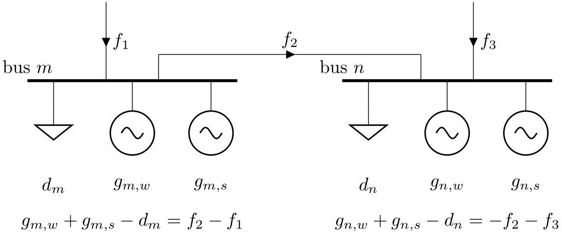
Nodal power balances#
This is the most important equation, which guarantees that the power balances at each bus \(n\) for each time \(t\).
Where \(d_{n,s,t}\) is the exogenous load at each node (load.p_set) and the incidence matrix \(K_{nl}\) for the graph takes values in \(\{-1,0,1\}\) depending on whether the branch \(l\) ends or starts at the bus. \(\lambda_{n,t}\) is the shadow price of the constraint, i.e. the locational marginal price, stored in network.buses_t.marginal_price.
The bus’s role is to enforce energy conservation for all elements feeding in and out of it (i.e. like Kirchhoff’s Current Law).
Global constraints#
Global constraints apply to more than one component.
Currently, five global constraint types are defined. They are activated if a
global constraint with the corresponding type is added to the network.
By default, the constraint applies to all investment periods. For multi-decade
optimisation, a global constraint can be set for one investment period only
(e.g. a \(\mathrm{CO}_2\) limit for a specific investment year) by specifying this in the
attribute investment_period. The shadow price of each global constraint is
stored in \(\mu\) which is an output of the optimisation stored in network.global_constraints.mu.
Primary Energy#
The primary energy constraints (type=primary_energy) depend on the power plant efficiency and carrier-specific attributes such as
specific \(\mathrm{CO}_2\) emissions.
Suppose there is a global constraint defined for \(\mathrm{CO}_2\) emissions with
sense <= and constant \(\textrm{CAP}_{CO2}\). Emissions can come
from generators whose energy carriers have \(\mathrm{CO}_2\) emissions and from
stores and storage units whose storage medium releases or absorbs \(\mathrm{CO}_2\)
when it is converted. Only stores and storage units with non-cyclic
state of charge that is different at the start and end of the
simulation can contribute.
If the specific emissions of energy carrier \(s\) is \(e_s\)
(carrier.co2_emissions) \(\mathrm{CO}_2\)-equivalent-tonne-per-MWh and the
generator with carrier \(s\) at node \(n\) has efficiency
\(\eta_{n,s}\) then the \(\mathrm{CO}_2\) constraint is
The first sum is over generators; the second sum is over stores and storage units. \(\mu\) is the shadow price of the constraint, i.e. the \(\mathrm{CO}_2\) price in this case.
Transmission Volume Expansion Limit#
This global constraint can limit the maximum line volume expansion in MWkm
(type=transmission_volume_expansion_limit). Possible carriers are ‘AC’ and ‘DC’.
Transmission Expansion Cost Limit#
This global constraint can limit the maximum cost of line expansion
(type=transmission_expansion_cost_limit). Possible carriers are ‘AC’ and ‘DC’.
Technology Capacity Expansion Limit#
This global constraint can limit the maximum summed capacity of active assets
of a carrier (e.g. onshore wind) for an investment period at a chosen node
(type=tech_capacity_expansion_limit).
This constraint is mainly used for multi-decade investment planning. It can represent land
resource or building rate restrictions for a technology in a certain region.
Currently, only the capacities of extendable generators have to be below the set limit.
For example, the capacities of all onshore wind generators (carrier_attribute="onshore wind") at a certain bus
(bus="DE") should be smaller (sense="<=") than the technical potential for onshore wind
in the specific region (constant=Limit). Then the technology capacity expansion constraint is
Where \(A\) are the investment periods, \(s\) are all extendable generators of the specified carrier, \(b_s\) is the build year of an asset \(s\) with lifetime \(L_s\).
The constraint can also be formulated with the opposite sense, so that, a minimum expansion of a certain technology is required on a certain bus.
Operational Limit#
Warning
Be aware, this global constraint type is only implemented in linopy and only activated when calling n.optimize.
This global constraint can limit the net production of a carrier taking into
account generator, storage units and stores (type=operational_limit).
Optimising investment and operation over multiple investment periods#
In general, there are two different methods of pathway optimisation with perfect foresight. These differ in the way of accounting the investment costs:
In the first case (type I), the complete overnight investment costs are applied.
In the second case (type II), the investment costs are annualised over the years, in which an asset is active (depending on the build year and lifetime).
Method II is used in PyPSA since it allows a separation of the discounting over different years and the end-of-horizon effects are smaller compared to method I. For a more detailed comparison of the two methods and a reference to other energy system models see https://nworbmot.org/energy/multihorizon.pdf.
Note
Be aware, that the attribute capital_cost represents the annualised investment costs
NOT the overnight investment costs for the multi-investment.
Multi-year investment instead of investing a single time is not implemented via the old optimization with n.lopf(pyomo=True).
It can be passed by setting the argument
multi_investment_periods when calling the
network.optimize(multi_investment_periods=True). For the pathway
optimisation snapshots have to be a pandas.MultiIndex, with the first level
as a subset of the investment periods.
The investment periods are defined in the component investment_periods.
They have to be integer and increasing (e.g. [2020, 2030, 2040, 2050]).
The investment periods can be weighted both in time called years
(e.g. for global constraints such as \(\mathrm{CO}_2\) emissions) and in the objective function
objective (e.g. for a social discount rate) using the
investment_period_weightings.
The objective function is then expressed by
Where \(A\) are the investment periods, \(w^o_a\) the objective weighting of the investment period, \(b_s\) is the build year of an asset \(s\) with lifetime \(L_s\), \(c_{s,a}\) the annualised investment costs, \(o_{s,a, t}\) the operational costs and \(w^\tau_{s,a}\) the temporal weightings (including snapshot objective weightings and investment period temporal weightings).
The general procedure for modelling multi-investment periods in PyPSA is to add
an asset for each investment period, in which its capacity should be expandable.
For example, if you want to optimise onshore wind development in the period 2025-2040
with investment periods every 5 years, you add a generator with a corresponding
construction year and lifetime for each investment period
(onwind-2025, onwind-2030, onwind-2035, onwind-2040).
This allows one to specify different technological assumptions for the respective
investment period (for example, decreasing investment costs, increasing efficiencies,
improved capacity factors due to higher hub heights of wind turbines, extended lifetimes).
The generators are only available for use after the year of construction and before
the end of their lifetime, for example, the onwind-2030 generator built in 2030
cannot contribute to electricity generation in the 2025 investment period.
To ensure that the technical potential for onshore wind in the region is not
exceeded by the 4 onshore wind generators in our example, one has to add an
additional global constraint (type=tech_capacity_expansion_limit, see further description above).
Note that the capital_cost of the assets is now the fixed annual costs, including annuity and FOM.
Example jupyter notebook for multi-investment and python
script examples/multi-decade-example.py.
Useful constraints for multi-investment optimisation#
Growth Limit per Carrier#
A growth limit per carrier which constraints new installed capacities for each
investment period can be defined by setting the attribute max_growth for the
PyPSA component carrier.
Technology Capacity Expansion Limit#
See above description in Global Constraints for Technology Capacity Expansion Limit.
\(\mathrm{CO}_2\) targets for single investment periods#
This can be implemented via a global primary energy constraint, see above description for Primary Energy Constraint.
Abstract problem formulations#
Through the pypsa.optimization.abstract module, PyPSA provides a number of problem formulations that can be used to solve different types of power system optimisation problems. The following problem formulations are currently available:
Iterative transmission capacity expansion#
If the transmission capacity is changed in passive networks, then the impedance will also change (i.e. if parallel lines are installed). This is not reflected in the ordinary optimization, however Network.optimize.optimize_transmission_expansion_iteratively covers this through an iterative process as done in here.
Security-Constrained Power Flow#
To ensure that the optimized power system is robust against line failures, security-constrained optimization through Network.optimize.optimize_security_constrained enforces security margins for power flow on Line components. See Contingency Analysis for more details.
Custom constraints and other functionality#
Custom constraints are important because they allow users to tailor optimization problems to specific requirements or scenarios. By adding custom constraints, users can model more complex or realistic situations that may not be captured by the default optimization formulations provided by PyPSA.
To build custom constraints, users can access and modify the Linopy model instance associated with the PyPSA network. This model instance contains all variables, constraints, and the objective function of the optimization problem. Users can directly add, remove, or modify variables and constraints as needed.
Given a network n and the corresponding model instance m, some key functions used in the code for working with custom constraints include:
n.optimize.create_model(): Creates a Linopy model instance for the PyPSA network.m.variables[](): Accesses the optimization variables of the Linopy model instance.m.add_variables(): Adds custom variables to the Linopy model instance.m.add_constraints(): Adds custom constraints to the Linopy model instance.n.optimize.solve_model(): Solves the optimization problem using the current Linopy model instance and updates the PyPSA network with the solution.
A typical workflow starts with creating a Linopy model instance for a PyPSA network using the n.optimize.create_model() function. This model instance contains all the optimization variables, constraints, and the objective function, which can be accessed and modified to incorporate custom constraints.
>>> m = n.optimize.create_model()
This will create a Linopy model instance m for the PyPSA network n and is also accessible using the n.model attribute. Accessing and combining variables is an essential part of creating custom constraints. You can access variables using the Linopy model instance’s variables attribute, which provides a dictionary-like structure containing the variables associated with each component in the network. For example, you can access generator active power variables using:
>>> gen_p = m.variables["Generator-p"]
This will return an array of variables, of class linopy.Variable which defines a variable reference for each generator and snapshot in the network. The Variable type is closely related to xarray.DataArray and pandas.DataFrame, and can be used in similar ways. To create custom constraints, you may need to combine variables, such as generator output and line flow variables, using mathematical operations like addition, subtraction, multiplication, and division.
When defining a custom constraint, you can create a Linopy expression representing the relationship between the variables involved in the constraint. The expression can be created using standard Python operators like ==, >=, and <=. For example, if you want to create a constraint that forces the total generation at a bus to be at least 80% of the total demand, you can create an expression like:
>>> bus = n.generators.bus.to_xarray()
>>> total_generation = gen_p.groupby(bus).sum().sum("snapshot")
>>> total_demand = n.loads_t.p_set.sum().sum()
>>> constraint_expression = total_generation >= 0.8 * total_demand
Note that in the Linopy formulation variable expressions stand on the left-hand-side of the constraint, while the right-hand-side is a constant value. After defining the custom constraint expression, add it to the Linopy model using the m.add_constraints() function, providing a name for the constraint to facilitate further modifications or analysis:
>>> m.add_constraints(constraint_expression, name="Bus-minimum_generation_share")
Once you have added your custom constraints to the Linopy model, use the n.optimize.solve_model() function to solve the optimization problem. This function considers your custom constraints while solving the optimization problem and updates the PyPSA network with the resulting solution:
>>> n.optimize.solve_model()
By following this workflow, you can create and modify optimization problems with custom constraints that better represent your specific requirements and scenarios using PyPSA and Linopy.
Note that alternatively the extra_functionality argument can be used in the optimize function to add custom functions to the optimization problem. The function is called after the model is created and before it is solved. It takes the network and the snapshots as arguments. However, for ease of use, we recommend using the workflow described above.
Further examples can be found in the examples section of the PyPSA documentation and in the Linopy documentation.
Fixing variables#
It is possible to fix all variables to specific values. Create a pandas DataFrame or a column with the same name as the variable but with suffix ‘_set’. For all not NaN values additional constraints will be build to fix the variables.
For example let’s say, we want to fix the output of a single generator ‘gas1’ to 200 MW for all snapshots. Then we can add a dataframe p_set to network.generators_t with the according value and index.
>>> network.generators_t['p_set'] = pd.DataFrame(200, index=network.snapshots, columns=['gas1'])
The optimization will now build extra constraints to fix the p variables of generator ‘gas1’ to 200. In the same manner, we can fix the variables only for some specific snapshots. This is applicable to all variables, also state_of_charge for storage units or p for links. Static investment variables can be fixed via adding additional columns, e.g. a s_nom_set column to network.lines.
Inputs#
For the linear optimal power flow, the following data for each component are used. For almost all values, defaults are assumed if not explicitly set. For the defaults and units, see Components.
network.{snapshot_weightings}
bus.{v_nom, carrier}
load.{p_set}
generator.{p_nom, p_nom_extendable, p_nom_min, p_nom_max, p_min_pu, p_max_pu, marginal_cost, capital_cost, efficiency, carrier}
storage_unit.{p_nom, p_nom_extendable, p_nom_min, p_nom_max, p_min_pu, p_max_pu, marginal_cost, capital_cost, efficiency*, standing_loss, inflow, state_of_charge_set, max_hours, state_of_charge_initial, cyclic_state_of_charge}
store.{e_nom, e_nom_extendable, e_nom_min, e_nom_max, e_min_pu, e_max_pu, e_cyclic, e_initial, capital_cost, marginal_cost, standing_loss}
line.{x, s_nom, s_nom_extendable, s_nom_min, s_nom_max, capital_cost}
transformer.{x, s_nom, s_nom_extendable, s_nom_min, s_nom_max, capital_cost}
link.{p_min_pu, p_max_pu, p_nom, p_nom_extendable, p_nom_min, p_nom_max, capital_cost}
carrier.{carrier_attribute}
global_constraint.{type, carrier_attribute, sense, constant}
Outputs#
bus.{v_mag_pu, v_ang, p, marginal_price}
load.{p}
generator.{p, p_nom_opt}
storage_unit.{p, p_nom_opt, state_of_charge, spill}
store.{p, e_nom_opt, e}
line.{p0, p1, s_nom_opt, mu_lower, mu_upper}
transformer.{p0, p1, s_nom_opt, mu_lower, mu_upper}
link.{p0, p1, p_nom_opt, mu_lower, mu_upper}
global_constraint.{mu}